How To Analyze and Adjust
Downstream Control Operation

Introduction

Downstream Control Operation is possibly the most complex piece of the release decision logic in HEC-ResSim, and a lot goes on behind the scenes that many users either do not know about or do not know how to analyze and influence. The objective of this document is to describe some of what is going on, show you how to find and analyze some of the diagnostic output, and explain the various options and settings that you can use to influence the operations.

Some Basics

The Downstream Control Function rule is how you call for the downstream control operation in ResSim. When creating this rule, you must specify the "control point" – the location where rule's limit is applied. Then you define the parameter (flow or stage), the limit type (min or max), and the function that describes the limit. Once you have completed the definition of the limit function, you add the rule to the appropriate zones of the reservoir and prioritize the rule with other rules in each zone.

What ResSim is going to do next…

Determine the Routing Time Window

The Routing Time Window (or Number of Routing Steps) is the number of timesteps into the future that a release made in the current timestep affects the flow at the downstream location.

Pulse Flow Routing

Before the computations ever really get started, ResSim is going to analyze the operation set in each reservoir of your model looking for features that will trigger or influence various preparatory functions. One such function is the Evaluating Routing for Downstream Operations compute loop, which is triggered by downstream control rules. This function routes a "pulse flow" hydrograph from each reservoir that has a downstream control rule to the downstream-most junction of the network. ResSim then analyzes the routed pulse flow at each control point to determine an initial estimate of the routing time window for the operation for each control point and to produce a set of linear routing coefficients that would produce an equivalent routed pulse hydrograph.
Figure 1 below shows a plot of the pulse flow hydrograph as it leaves the reservoir (blue curve) and the routed pulse flow hydrograph at the control point (red curve).

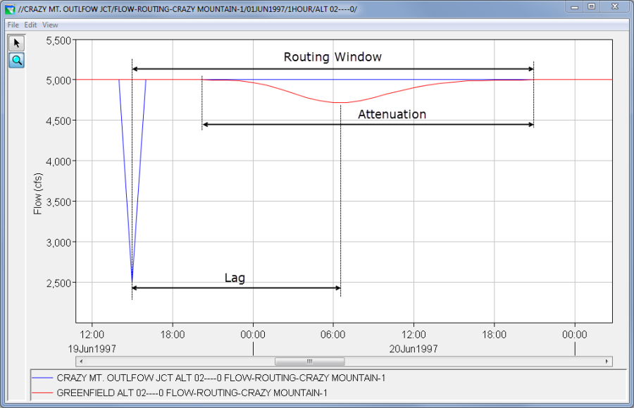
   Figure 1 – Pulse Flow routing

This plot illustrates some important concepts about the pulse routing logic in ResSim:

• Note the shape of the pulse flow hydrograph. The (default) pulse flow time series represents a constant value of 5000 cfs being release from the reservoir, which is cut back to 2500 cfs (½ * 5000) for one timestep. This "cut back" is the pulse of the pulse flow hydrograph. The reason for using an inverted pulse is to reflect the inertia of the water already in storage in the reach and the response to a single significant perturbation – a bit like the ripples caused by a drop of water on a still pond.
• Next, note the shape and position of the routed pulse hydrograph. The inverted peak of the routed hydrograph should occur after the inverted peak of the pulse and no portion of the routed pulse hydrograph should exceed the constant flow value of the pulse hydrograph.
• The annotations added to the plot identify what ResSim considers the lag and attenuation due to routing. Also identified is the routing window – which starts at the peak of the pulse flow hydrograph and ends at the end of the attenuation of the routed pulse hydrograph.

Although Figure 1 is good for illustrating the lag, attenuation, and routing window as interpreted by ResSim, it represents an ideal situation. Less than ideal situations are not unusual, and some can result in poor operation for the downstream control objective or excessively long compute times. Figure 2 illustrates an unstable pulse routing situation in which the routed pulse hydrograph (red) oscillates across the constant flow of the original pulse (blue). An additional curve has been added to illustrate the routed hydrograph for the same location but with the routing parameters adjusted to eliminate the instability (green).

Figure 2 – Stable and Unstable Pulse routing 

Use the Routing Window

The downstream control logic in ResSim uses the routing window as the size of an internal iteration loop. At the start of this loop, ResSim uses the lag, attenuation, and linear routing parameters to make an estimate of the release that it should make to meet the downstream objective, then it computes forward through the timesteps of the routing window loop to determine if the release it made in the first timestep of the loop violates the objective during the loop; if it identifies a violation, it makes an adjustment to improve the operation and runs through the loop one more time to verify the adjustment had the desired effect.
Figure 3 shows the results of the downstream control operation at the control point using the two sets of routing for the reach illustrated in Figure 2. The annotations in Figure 3 show how the unstable routing can produce inadequate downstream operation for the control point as well as some subtle clues that the routing may be unstable.

Figure 3 – Results of routing on downstream operation

What You Can Do To Improve Your Downstream Operation…

• Set the Value of the Pulse Flow for Each Reservoir
• Check the Pulse Routing Results and Adjust your Routing Parameters as Needed
• Use the Downstream Control Rule's Advanced Options

Set the Value of the Pulse Flow for Each Reservoir

The default constant value for the pulse flow hydrograph is 5000 cfs. If you are using a linear routing method, such as Muskingum, this value is adequate. However, if you are using a non-linear routing method, then you should adjust the constant value of the pulse flow to reflect the flow regime of your downstream control limit. To edit the Pulse Flow Hydrograph's constant value:

• Open the Reservoir Editor
• Select the Physical tab
• Select the Dam element in the Reservoir tree
• Right-click on the Dam element or open the Dam menu and select Pulse Flow Options
• The Pulse Routing Options dialog will open. In the table below the Default Pulse Flow text box, uncheck the Use Default checkbox and enter a new Pulse Flow value for each reservoir in your network that you want to revise. Use a value equal to 1-1.5 time greater than the downstream control rule's limit value.

 Figure 4 Pulse Routing Options Dialog

NOTE – ResSim only uses one estimate of the routing for all downstream control rules for a given control point. That means that if you have both minimum and maximum rules for a given downstream location, you must determine which rule(s) are most import to your analysis, the downstream minimum or the downstream maximum; and that's the limit you want to use for the pulse flow value.

Check the Pulse Routing Results and Adjust your Routing Parameters as Needed.

To determine if your routing is stable and is producing a reasonable routing window, you should prepare plots similar Figures 1 & 2 above. To do so:

• Open a simulation in which you have computed an alternative with an active downstream control rule.
• Open DSSVue from the Tools menu; the simulation.dss file for the current simulation will open automatically.
• Filter the pathname list using a C-part of FLOW-ROUTING-reservoirName where reservoirName is the name of the reservoir that has the downstream control rule you are interested in.
• Select the time series for the reservoir outflow junction and the control point and plot them.
  • If your plot looks similar to Figure 1…
    • Review the plot carefully and estimate the lag time and the length of the routing window in timesteps.
    • Compare your estimate of the routing window to the estimate produced by ResSim. ResSim's estimate can be found in the Compute log. Search for the string "Pulse Width Steps = "; the value given in the message is the length of the routing window.

HOWEVER, if the "Pulse Width Steps = " message is followed by another message that begins with "Pulse Width Steps associated with ROC constraints = ", then the routing window reported in the first message has been lengthened due to the influence of Rate of Change constraints. To find ResSim's estimate of the routing window due only to routing, subtract the ROC value from the first reported routing window. If your estimate does not match ResSim's, zoom in more carefully on the tail of the routed hydrograph in your plot to see if you left out a few timesteps.

• • If your plot looks similar to Figure 2 (the routed pulse flow oscillates above the constant flow in the pulse flow hydrograph), your routing is unstable and you should make some adjustments to your routing parameters until you get a stable pulse routing plot.

    • If your model has several reaches between your reservoir's outflow junction and the downstream control point, the unstable routing you see at the control point could be caused by the routing of one or more of the intervening reaches. To identify which reaches are the source of the problem, try adding the FLOW-ROUTING time series for some or all of the junctions between the reservoir and the control point to your plot as illustrated in Figure 5. OR, treat each intervening junction as a control point and plot its FLOW-ROUTING time series with the reservoir outflow junction's and analyze each reach one at a time.

      Figure 5 – Pulse Routing PlOT for Multiple Junctions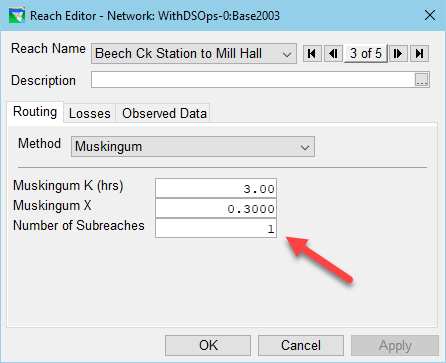

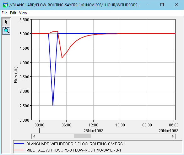
      Figure 6 – Pulse Routing Options Dialog

    • For most routing methods, properly adjusting the number of subreaches or substeps will usually take care of the problem. As a rule of thumb, the number of subreaches should equal the routing or lag time of the reach divided by the length of the compute interval rounded to the nearest whole number. For example, for the reach illustrated if Figure 6, the lag time of the reach is approximately 3 hours. If the compute interval in ResSim is 1 hour, then the number of subreaches should be equal 3/1 = 3. Using a value of 1 can cause an instability in the routing of this reach as illustrated in the pulse routing plot shown in Figure 7.

Use the Downstream Control Rule's Advanced Options

Several options are available in the Downstream Control Rule's Advanced Options Dialog. Each option has a unique impact on the downstream control operation.

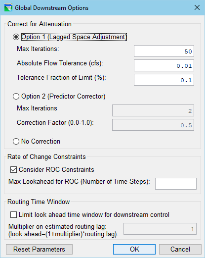
Figure 8 – Pulse Routing Options Dialog

Correct for Attenuation

The Options to correct for attenuation impact the "adjustment" that is made to each release estimate ResSim makes to meet the downstream objective. These options were added when it was discovered that the downstream control rule's decision logic was negatively impacted when the local inflows oscillated or varied significantly within the routing window. Option 1 seems to work well with non-linear routing. Option 2 seems to be work with linear routing. And the No Correction option seems to work best with Null or Linear routing with smoothly and gradually varied local flows.

Rate of Change Constraints

The downstream control logic includes a section for widening the routing window to allow rate of change constraints to be applied without violating the downstream constraint. This expansion of the routing window can sometimes be excessive and result in poor downstream operation and increased compute time. This Advanced Option allows you to limit the impact of Rate of Change constraints on the routing window. Your options are to turn off the impact altogether or to set a maximum number of time steps that can be added to the routing window to account for rate of change.

Routing Time Window

One of the most common "less than ideal" pulse routing situations that you should watch for is an extended tail on the routed pulse hydrograph. The extended tail can result in a routing window that is far too long and can result in invalid or unexplainable downstream operation as well as excessive compute time. Modifying the routing parameters is usually not the solution for this problem. Instead, you may want to limit the Routing Time Window. To do so:

• Review the pulse routing plot of the reservoir and control point's FLOW-ROUTING time series.
• Estimate the routing window that accounts for approximately 80-90% of the volume of the "under" the original pulse flow in the routed hydrograph. Then compute the ratio of your estimate to lag time of the routed pulse flow. The multiplier is that ratio minus one:

Multiplier = [80% Estimate]/[Lag] - 1.