HOW TO Run a Reservoir Pool Firm Yield Analysis with ResSim

The firm yield is the demand that can be just barely satisfied by inflow and storage through the driest period experienced (period of record hydrology) or expected (synthetic hydrology). Firm Yield is limited by a critical period which can vary based on the demand and storage capacity.

This example covers one way to conduct a firm yield analysis for a reservoir pool. Future documentation will describe other approaches and offer examples for doing water account yield analysis. To begin a firm yield analysis for a reservoir, an initial network and base alternative are needed, along with inflows for the period of record, or a comparable synthetic record. Typically, it is best to start with an existing alternative that has been shown to compute correctly through the period of record. These instructions assume that you are starting with an existing, well-reviewed watershed that contains an alternative that represents "current conditions".

Begin by identifying an existing network and alternative that represent the current conditions. This "base network" will begin as a copy of the current conditions network. Later, you will simplify this network and then add some physical and/or operational features to it. The "base alternative" is a new alternative created for the base network but using the current conditions alternative as a template. You will use the base alternative to test that the model is running as expected before adding the yield operation.

Create a Base Network for the Yield Analysis

In the Reservoir Network module, open the current conditions network.
From the Network menu, select Save As… to create a copy of the current conditions network ("Figure: New Network"). Give the new network an appropriate name.

Figure: New Network

Create a Base Alternative for the Yield Analysis

Next, create a new alternative based on the new network ("Figure: Alternative Editor - New Alternative"). This alternative will be the base alternative for all the yield alternatives you may create.
Figure: Alternative Editor - New Alternative
Copy the setup of the existing current conditions alternative into the new alternative—this is easier to do if you haven't made any changes to the network yet.
Start with the Run Control tab. Set the Time Step and the Flow Computation Method to the same settings as in the template (current conditions) alternative. Set the Alternative Type to Standard. Also, consider the settings for Compute Unregulated Flow and Compute Holdouts. You obviously will not need Holdouts for this alternative and you probably won't need Unregulated Flows either (unless there's something in the operations that uses them); if you can, set both of these options to OFF (unchecked) so that their computes do not add unnecessarily to the compute time of each iteration of your alternative.
Next, on the Operations tab, set the Operation Set for each reservoir in the network using the same settings as those in the template alternative.
On the Lookback tab, copy the settings for each entry in the table from your template alternative to your new alternative, then Save the alternative before moving on to the Time Series tab. You do not need the Observed data in your yield alternatives, so don't copy that information. However, if you limited the output generated by ResSim using the DSS Output tab in your template alternative, consider copying those settings, too.
When you are done copying the data from the template alternative to the new alternative, save the new alternative and close the Alternative Editor.
Change to the simulation module and create a new period of record simulation with the same time window as a simulation in which your current conditions alternative was used. Include only the new alternative in the new simulation.
Compute the new alternative. Be sure to use the Save to Base Directory… option if you have to make any changes to get the alternative working and computing properly.

When you need to make a copy of an alternative but Save As is not an option (usually when the new alternative uses a different network than the original alternative), use the following steps to simplify the process of copying the table data from one alternative to another:

In the Alternative Editor, select the old alternative, then select the tab with the table you want to copy from.
Click in the first cell of the table (the upper-left-most cell), then press… Ctrl+A—to select all the rows and columns, then press Ctrl+C—to copy your selection to the Windows® clipboard
Now, select the new alternative
Click in the first cell of the table you want to copy the data to, then press… Ctrl+V—to paste the data you copied into the table.

Repeat these steps for each tab and table of the alternative you want to copy.
*When using this shortcut, be sure the tables you are copying from and pasting to match row by row. When the new network is an unchanged copy of the original network, you can ensure matching fields by first copying the data from/to the Operations tab and the Lookback tab and then saving the alternative, before copying the data from/to the Time-Series tab.

Add Physical Elements Needed for the Yield Analysis

Return to the Reservoir Network module.
Consider adding a diverted outlet for water supply ("Figure: Define the Diverted Outlet") to the yield reservoir(s). See .Diverted Outlets v3.5 for instructions on adding a diverted outlet to a reservoir. Note that depending on the nature of your system and analysis, a diverted outlet may or may not be useful to conducting a firm yield analysis. You can alternatively apply the water supply specified release rule to the existing outlets. Considerations for whether or not to use a diverted outlet include: whether demand is taken directly from the pool or downstream, how many reservoirs have water supply demands, and how other operations interact with the water supply yield.

Figure: Define the Diverted Outlet

Create a Base Operation Set for the Yield Analysis

Figure: Duplicate Reservoir Operation Set

In each yield reservoir, make a base operation set for use in your yield alternative(s) by duplicating the operation set used to represent current conditions ("Figure: Duplicate Reservoir Operation Set").
Next, remove rules in the yield operation set to reflect only the constraints that must exist at the same time as the demand. It may be appropriate to remove most, if not all, rules from the reservoirs. Note that a complete analysis may then involve adding the rules back into the operations to examine all system interactions.
If you created any diverted outlets to represent the withdrawals that you are going to maximize, add a rule to keep the diverted outlet closed when not needed to meet demand. This can be accomplished with a low priority maximum release rule of zero flow applied to the diverted outlet ("Figure: Max of Zero Rule on Diverted Outlet"). When the water supply demand rule is added, it will be placed above the max of zero rule so that the diverted outlet will only release to meet demand.
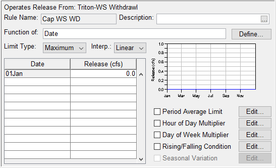Figure: Max of Zero Rule on Diverted Outlet
Close the Reservoir Editor and Save the network.

Update and Verify the Base Alternative

Open the Alternative Editor and select the base alternative.
On the Operations tab, select the new base yield operation sets for each yield reservoir.
On the Lookback tab, set the Lookback Release of the diverted outlet(s) to a constant of zero flow. Set the Lookback Storage to the top of the guide curve; this assumes that the critical period is not during the start of the period of record. Make sure your alternative is using the correct inflows.
Save the alternative and close the Reservoir Editor.
Change back to the Simulation module and the period of record simulation you created.
Right-click on your alternative in the Simulation Control Panel and select Replace from Base from the context menu to update the alternative with the changes you just made in the Network module.
Compute the alternative and verify that it is still computing correctly.

Create a Yield Analysis Alternative

Once a base alternative has been created and is running correctly, a Yield Analysis alternative can be developed. The following instructions assume that you are going to perform a Firm Yield analysis on the existing conservation pool of a reservoir in your network. To do so:

Return to the Reservoir Network module. Make sure your yield network is the active network.
Open the Reservoir Editor and select the reservoir for which you will be computing the yield.
Duplicate your base operation set. In the example shown in "Figure: Reservoir Editor - New Operation Set and New Yield rule", the new operation set has been labeled Max Yield.
Create a specified Release Function rule and apply it to the diverted outlet (or dam or other outlet, as necessary). This rule will represent the water supply demand to be maximized.
Give the new demand rule a starting value or seasonal pattern. This value will be replaced during each iteration of the Yield Analysis run.

Add the demand rule to the zone(s) that make up the conservation pool. Also, add this rule to the adjacent zones above and below the conservation pool. If the lower adjacent zone is the Inactive zone, then the rule only needs to be added to the zone immediately above the guide curve (typically the Flood Control zone). In the example shown in "Figure: Reservoir Editor - New Operation Set and New Yield rule", the new rule is called "WS Yield" and has a starting value of 50 cfs.

Figure: Reservoir Editor - New Operation Set and New Yield rule

In the Alternative Editor, use Save As… to make a copy of the base alternative ("Figure: Alternative Editor - Save As..."), then perform the following changes to create a yield alternative.
Figure: Alternative Editor - Save As...
On the Run Control tab, change the Alternative Type to Yield Analysis "Figure: Set Alternative Type to Yield Analysis". This will activate the Yield Analysis tab of the Alternative Editor.
Figure: Set Alternative Type to Yield Analysis
On the Operations tab, select the yield operation set you just created with your new yield rule ("Figure: Alternative Editor - Operations Tab - Select the Yield Operation Set(s)"). Save your alternative.
Figure: Alternative Editor - Operations Tab - Select the Yield Operation Set(s)
On the Yield Analysis tab ("Figure: Alternative Editor - Yield Analysis - Select the Rule and Set the Tolerances"), set the Yield Analysis Type to Reservoir Yield.
Figure: Alternative Editor - Yield Analysis - Select the Rule and Set the Tolerances
Use the radio buttons to select the Type of Demand Rule you are going to Maximize. Choose Water Supply Rules.
Select the Rule. The filters are provided to help you find the rule quickly. The list of available rules will only be long if the selected operation sets for your reservoirs are complex. To select the rule, you must highlight it and press the Select button.
Your selected rule will appear in the Selected Demand Rule table. Enter a flow Tolerance value for the rule. The flow tolerance is the maximum amount that the demand can be shorted and still pass the flow convergence test.
Storage information about the selected rule and its reservoir will appear in the storage table. Select the top-of-zone curve that marks the bottom of the pool from which the withdrawal defining the firm yield may be made.
Specify a storage Tolerance. The storage tolerance is the maximum amount of storage that may remain the reservoir conservation pool and still pass the storage convergence storage test.
Next, enter a Maximum number of Iterations. The default value is 25. Very few models require 25 iterations. If the compute has not converged within 25 iterations, you may have a problem with your model; review the Storage Yield report to determine if the iterations are oscillating away from solution or if one or both of tolerances are too small or too large.
The last parameter to set is the Convergence Method. Your options are Bisection Search Only and Heuristic and Bisection Search. The latter option allows you to specify how many Heuristic Iterations should be performed before automatically switching to Bisection Search Iterations.
Save your alternative.

Compute the Yield Alternative

Now that a Firm Yield alternative has been created, you can run it for the period of record.

In the Simulation Module, add your Firm Yield alternative to the period of record simulation that currently holds your base alternative.
Make your Firm Yield alternative the active alternative and compute it.

As each iteration completes, it reports how well it did with respect to the tolerances in the Compute Window and in the Compute Log. You can review these reported results while it runs or after it computes.

After the last iteration's status output, the final yield value will be reported. The final value for the maximized yield rule will also be stored in the demand rule itself. "Figure: Compute Window - Final Yield Value" shows the calculated yield value in the Compute Window.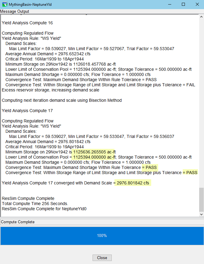
Figure: Compute Window - Final Yield Value
Open the Reservoir Editor to verify that the yield rule has been updated. "Figure: Reservoir Editor - Yield Rule - After Last Yield Iteration" shows that the simulation's copy of the yield alternative has the "WS Yield" rule populated with the same value.
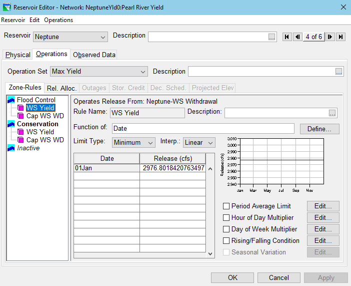
Figure: Reservoir Editor - Yield Rule - After Last Yield Iteration

Analyze the Yield Alternative Results