Download PDF
Download page Daily Average Record Extension - Yellowstone River.
Daily Average Record Extension - Yellowstone River
The Yellowstone_RecordExtension example demonstrates the usage of the Record Extension Analysis in order to extend a shorter daily average flow time series using a site with a longer period of record.
Input Data
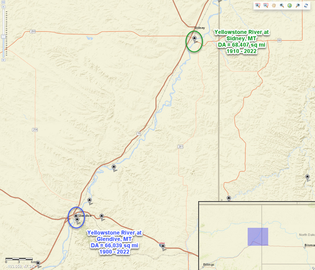
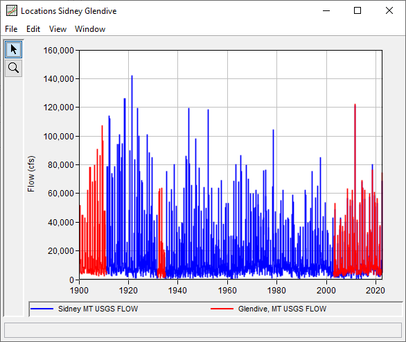
In this example, time series representing daily average flow at two locations within the Yellowstone River watershed in Montana are analyzed. The primary (i.e. long record) time series is from the Yellowstone River at Sidney, MT stream gage, which has a drainage area of approximately 68,407 square miles (sq mi) and a period of record from 1910 - 2022. The secondary (i.e. short record) time series is from the Yellowstone River at Glendive, MT stream gage, which has a drainage area of approximately 66,039 sq mi and a period of record from 1900 - 2022. However, the Glendive record has significant missing periods spanning 1911 - 1931 and 1934 - 2002. The location of these stream gages is shown in Figure 1. The time series are plotted within Figure 2.
General Tab
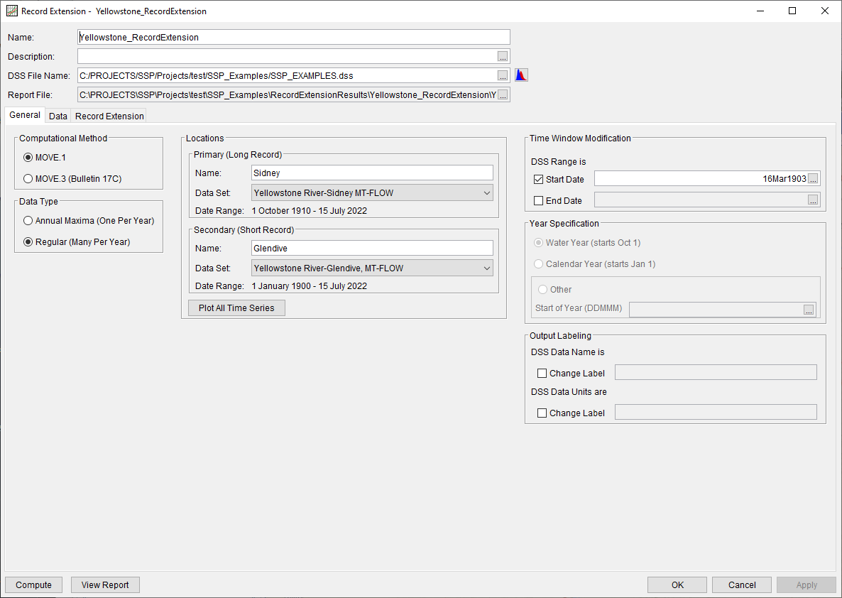
A Record Extension Analysis has been developed for this example. To open the analysis, either double-click on the analysis labeled Yellowstone_RecordExtension from the study explorer or from the Analysis menu select open, then select Yellowstone_RecordExtension from the list of available analyses. When Yellowstone_RecordExtension is opened, the General tab within the Record Extension Analysis editor will appear as shown in Figure 3. For this analysis, the MOVE.1 computational method and the Regular (Many Per Year) data type was selected. The Sidney time series was selected as the Primary (Long Record) while the Glendive time series was selected as the Secondary (Short Record). The time window was modified to start on 16Mar1903. No modifications were made to the year specification or the output labeling.
Data Tab
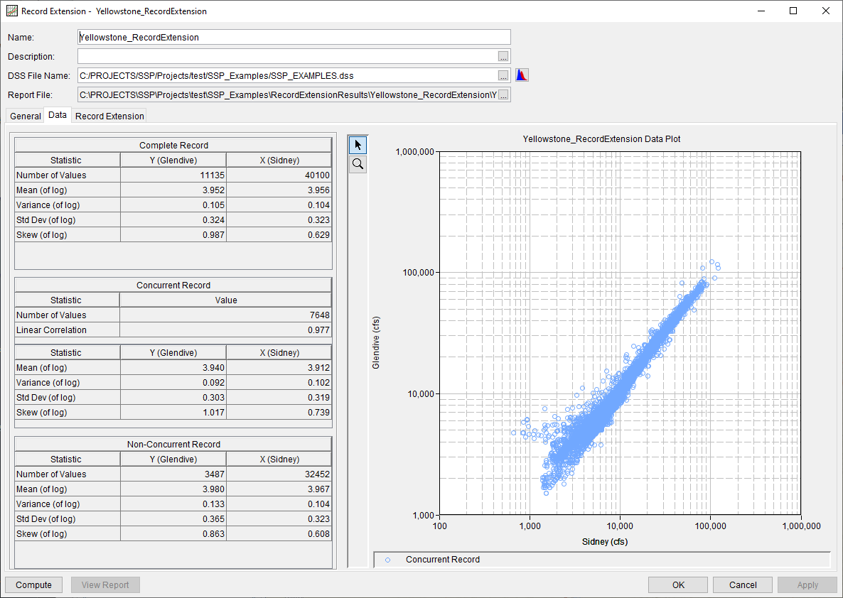
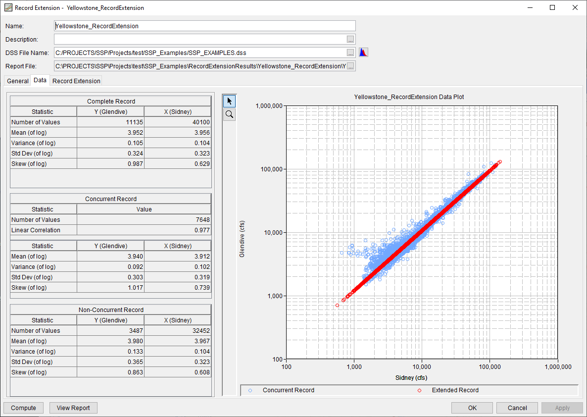
The Data tab contains several tables detailing the complete, concurrent (i.e. overlapping), and non-concurrent (i.e. non-overlapping) records. Additionally, a plot showing the concurrent record is included. The primary record (Scotia) is shown on the x-axis while the secondary record (Dos Rios) is shown on the y-axis. Prior to a successful compute, the plot will only contain the concurrent record (blue circles), as shown in Figure 4. Following a successful compute, the extended record (red circles) will be added to the plot, as shown in Figure 5.
Computing the Analysis
Once all of the General information has been selected and the data reviewed on the Data tab, the user can press the Compute button to perform the analysis. Once the computations have been completed, a message window will open stating Compute Complete.
Results Tab
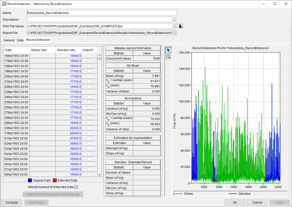
The Results tab contains several tables detailing the Matalas-Jacobs Estimators (MJ-Mean and MJ-Variance), the Estimators for Augmentation, and statistics of the extended record. Additionally, a plot showing the input time series is included. Prior to a successful compute, the plot will only contain the primary record (Sidney; green bars) and the secondary record (Glendive; blue bars), as shown in Figure 6. Following a successful compute, the extended record (red bars) will be added to the plot, as shown in Figure 7.
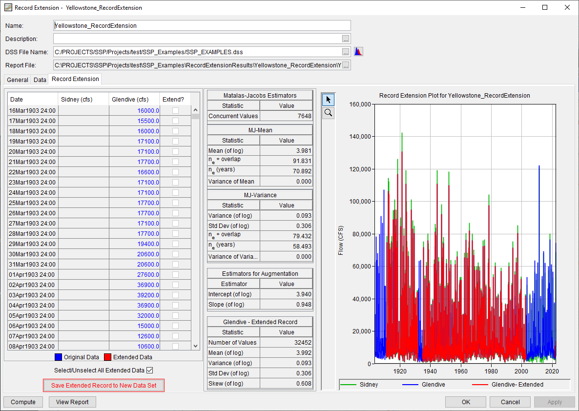
Since this example made use of the MOVE.1 computational method and the Regular (Many Per Year) data type, following a successful compute, the entire extended record will selected for extension and the Save Extended Record to New Data Set button will become enabled.
The Save Extended Record to New Data Set button will only be active following a successful compute.
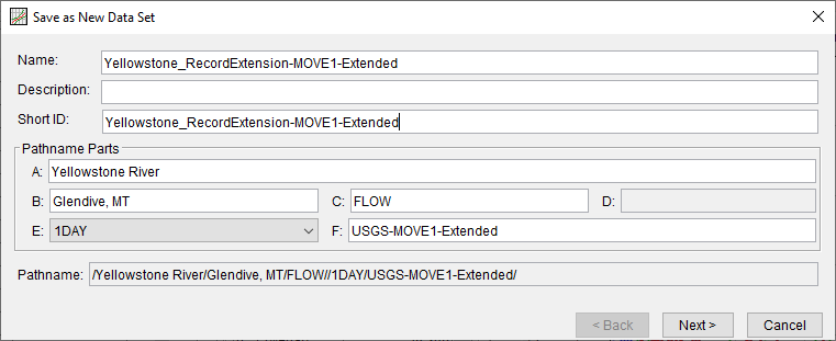
When the Save Extended Record to New Data Set is clicked, a dialog will be presented allowing for the definition of a Name, Description, Short ID, and DSS Pathname Parts for the new data set, as shown within Figure 8.
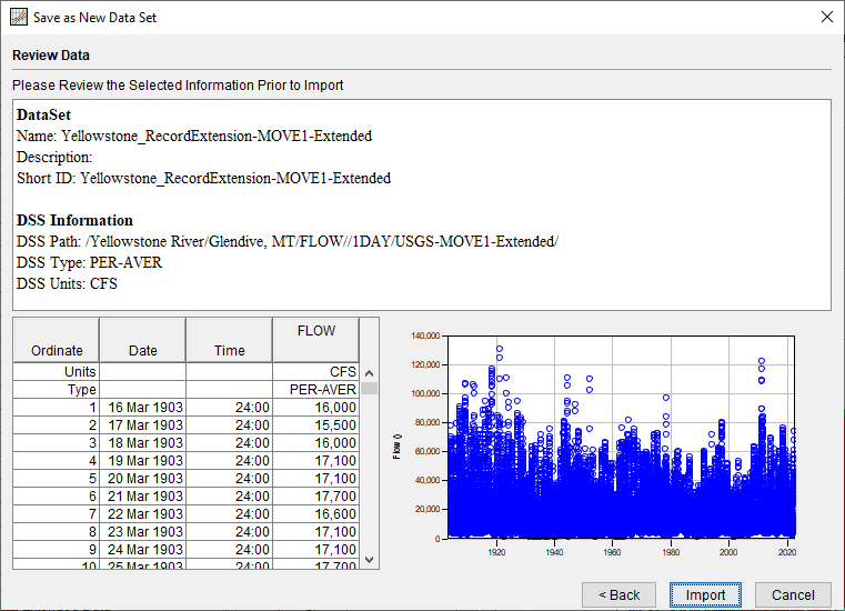
Upon clicking the Next button, a Save As New Data Set Summary dialog will be shown allowing the user to review the metadata of the new data set as well as a tabulation and plot of the data that is about to be imported, as shown in Figure 9.
Once the extended record is saved to a new data set, it can be used to compute updated flow-frequency and/or flow-duration information. An example of this type of application is shown here.
Report File
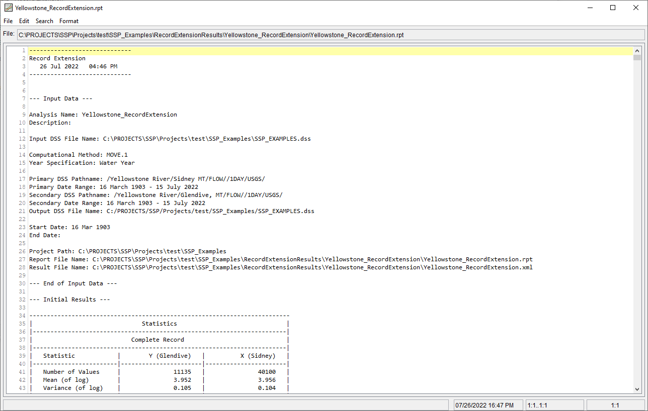
In addition to the tabular and graphical results, there is a report file that echoes the input data, selected computational options, and results. To review the report file, press the View Report button at the bottom of the analysis window. When this button is selected a text viewer will open the report file and display it on the screen, as shown in Figure 10.
Different types and amounts of information will show up in the report file depending on the data and the options that have been selected for the analysis.
