Daily Flow Record Extension with MOVE.1

Overview

This tutorial provides an example application of using the MOVE.1 record extension technique to estimate daily flow values using the Record Extension functionality. The record extension analysis uses data from a site with a long period of record to extend the flow dataset at a nearby site with a shorter period of record.

The MOVE.1 technique is not recommended for use when performing record extension on annual peak flow records. Bulletin 17C recommends the MOVE.3 approach in this case (England, et al, 2019). Refer to the previous example (Task 1. Create a new HEC-SSP Study and Import Data) for detail on how to perform a MOVE.3 extension using the Record Extension feature in HEC-SSP.

Download a copy of the initial HEC-SSP project here - MOVE1_Daily_Example_Initial.zip

Introduction

The MOVE.1 technique is often used for daily average flow record extensions. The MOVE.1 record extension technique was first proposed by Robert Hirsch in his 1982 paper, "A Comparison of Four Streamflow Record Extension Techniques". It is very similar to a simple ordinary least-squares (OLS) linear regression. The general equation for an OLS linear regression is below, written in a slightly different form from the familiar equation: y = mx + b. In our context, x is the streamflows at the long-term site and y is the streamflows at the short-term site over the concurrent period where both datasets exist:

$//<![CDATA[ \begin{array}{l}\hat{Y}_{i}=\bar{Y}+r\frac{S_{y}}{S_{x}}\left(X_{i} - \bar{X}\right)\end{array} //]]>$

The only difference between the OLS equation above and the MOVE.1 equation (shown below) is that the correlation term (r) is removed. This regression is also known as the Line of Organic Correlation. In the context of streamflow extensions, the correlation term (r) is usually between 0.7 and 1.0. Therefore, the MOVE.1 record extension makes the predictions at high flows higher than OLS and the predictions at low flows lower than OLS. 

$//<![CDATA[ \begin{array}{l}\hat{Y}_{i}=\bar{Y}+\frac{S_{y}}{S_{x}}\left(X_{i} - \bar{X}\right)\end{array} //]]>$

Before performing a MOVE.1 analysis on daily flows, the analyst must first consider the main question to be answered. Depending on the question at hand, the preferred analytical approach will change. MOVE.1 daily flow extensions are most appropriate when the primary purpose is to simply create a continuous, general purpose dataset. This may be needed for a long-term simulation of reservoir operations, or an assessment of hydropower potential. However, if the question at hand is focused on flood events or low-flow events, extreme care must be taken and a simple MOVE.1 analysis is rarely the best approach.

This tutorial first gives an example of performing a simple MOVE.1 record extension. The second example in this tutorial shows the dangers of using this record extension for flood hazard analysis, and suggests alternate approaches.  

Dataset Overview

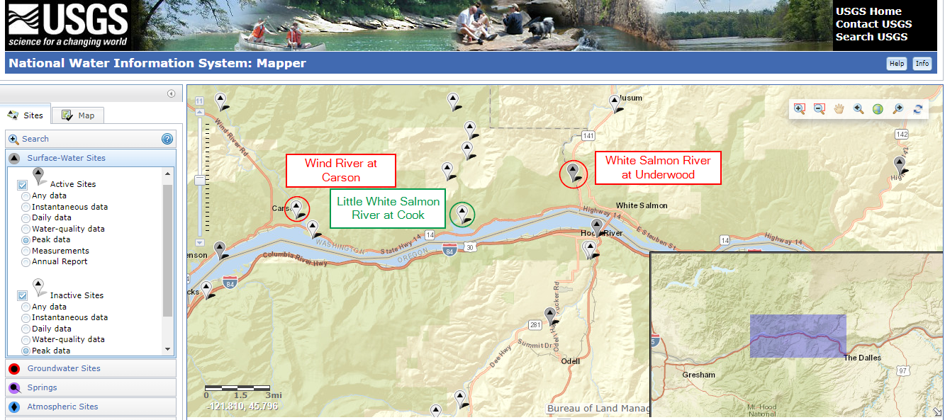
For this example, we will extend the record at the Little White Salmon River at Cook, which is a tributary to the Columbia River in southern Washington. It has a period of record of 1956-1977. Candidate nearby gages for the record extension include the Wind River at Carson and the White Salmon River at Underwood. 

Note: there are a few other inactive USGS gages on the Little White Salmon that include a few years of flow records before 1956. For the sake of this example, these sites are assumed not to exist for simplicity. If these datasets were used, they would be used to perform the first round of record extension, and then another round would be undertaken to fill in the rest of the dataset. 

Example 1: Daily flow record extension

To extend the daily flow record at Cook, a long-term gage must be selected first. If a correlation analysis is performed on annual peak flows, the correlation with the Carson gage (0.916) is higher than the Underwood gage (0.846). See Using a Correlation Analysis to Select a Suitable Nearby Gage for Record Extension tutorial for an example of performing a correlation analysis.

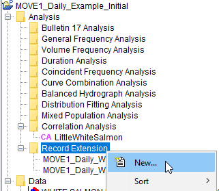
This might suggest that we should use the Carson gage to do the record extension. Let's check it out. Open the SSP project, and create a new Record Extension by right clicking on the folder. 

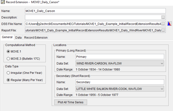
Name the analysis something like "MOVE1_Daily_Carson". Fill in the General tab as shown to set up the MOVE.1 analysis, and press the Compute button. 

Repeat these steps to create another MOVE.1 record extension based on the White Salmon at Underwood gage. Navigate to the "Data" tab to see how well the MOVE.1 record extension equation matches with the observed data. See the figures below for the results. Note that the Cook gage has a higher correlation with the Underwood gage than with the Carson gage (0.853). This is opposite of the correlation findings for the annual maximum peak flows. 

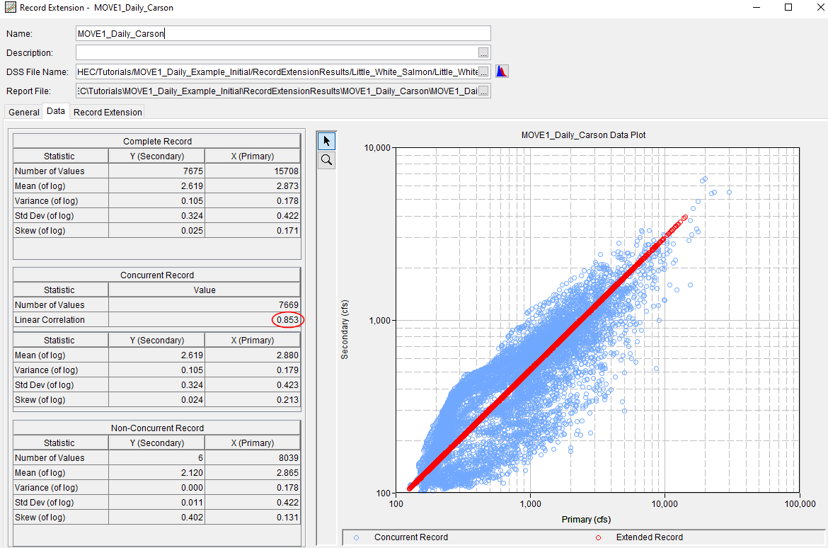
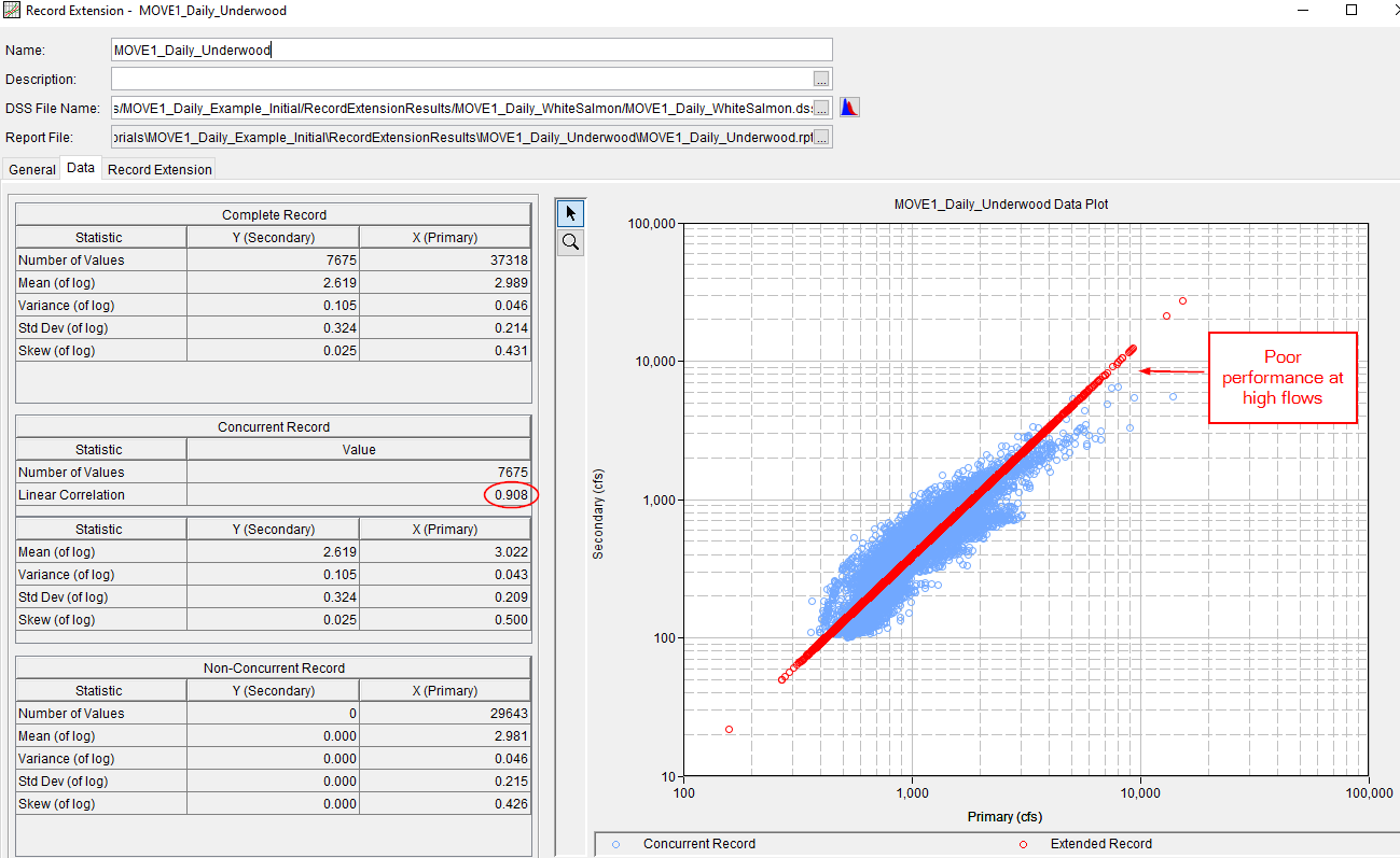
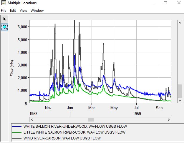
What's going on here? These three gages are in watersheds directly adjacent to each other. A plot of the daily flow data for water year 1959 is shown below for all three sites. It is apparent that the basin response to precipitation events is much more pronounced for the Wind River than the White Salmon and Little White Salmon rivers, where there appears to be much more groundwater interaction. For instance, the Carson gage shows a sizeable bump in flow near the beginning of May 1959, while the Cook gage barely registers an immediate increase. The recession limb during the summer is much more gradual for the Cook gage and the Underwood gage than the Carson gage. If flows during the summer are of primary concern, the Underwood gage is much more predictive than the Carson gage. But the regression plot above shows that the MOVE.1 regression with the Underwood gage is a poor predictor of high flows at Cook.

For this example, we'll assume that flood events are not of high concern, so we'll use the Underwood gage to finalize the daily record extension. Open the Record Extension you created with the Underwood gage, and navigate to the Record Extension tab. The thumbnail plot on the right shows the original datasets, as well as the extended records in red. To accept this record extension, click Save Extended Record to New Data Set. Give it a name, such as "Cook_Underwood-Extended". Click OK. Note that the extended dataset is listed in the main SSP window. 

Example 2: Application to Flood Volume Frequency Analysis

For this example, our goal is to produce flood volume frequency curves (e.g. 1-day, 3-day, 5-day, etc) at the Little White Salmon at Cook location. It is tempting to simply take the extended daily record calculated using MOVE.1, and perform a volume-frequency analysis on that dataset. However, this is typically only the best course of action when the correlation between the sites is extremely high. We'll take a look at this in this example and discuss alternatives.

As we previously saw, the daily average MOVE.1 extension of the Cook gage using the Underwood gage performs very poorly at high flows. We will use the Carson gage to perform the record extension instead. In SSP, repeat the same steps as previously detailed to generate a MOVE.1 daily extended record based on the Carson gage. Name it something like "Cook_Carson-Extended." Make sure to give the extended record a different DSS F-part so it doesn't overwrite the extension we did previously. This expands the record length from 22 years (1956-1977) to 43 years (1935-1977).

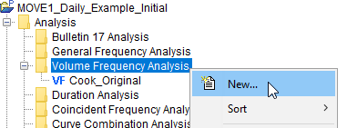
Now, we'll create two volume-frequency analyses–one with the original record, and one with the extended record. 22 years of record is too short for a volume-frequency analysis, but we'll look at it anyways for the sake of the example. Right click on the Volume Frequency Analysis folder, and select New.

Give your analysis a name, such as "Cook_Original", and for the Flow Data Set drop down box, select the original dataset (LITTLE WHITE SALMON RIVER-COOK, WA-FLOW). Keep most of the default settings except for the following:

1. In the General Tab, change the End Date of the Time window to end on 30Sep1977. The original daily flow dataset at Cook extends a few days into the beginning of October 1977. If we did not include this step, SSP will attempt to compute maximum volumes for water year 1978 using only this tiny amount of data.
   
   
2. Navigate to the Duration Table tab and click the Extract Volume-Duration Data button.
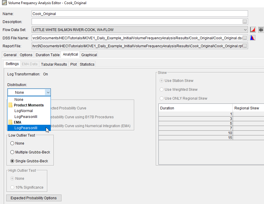
3. Navigate to the Analytical tab and then the Settings sub-tab. Change the Distribution to EMA | LogPearsonIII.
   
4. Press the Compute button at the bottom of the editor and look at the results.

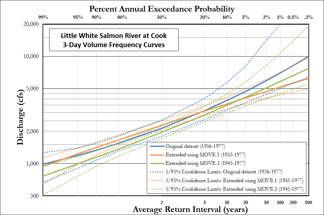
Repeat this process using the daily extended record based on the Carson gage. The two volume-frequency curves are shown below. Note how the addition of the extended record greatly reduced the skew of the curve. At the 1% annual exceedance probability (100-year) event for the 3-day duration, the original curve computed a value of 7000 cfs, while the extended record computed a value of 5200 cfs. 

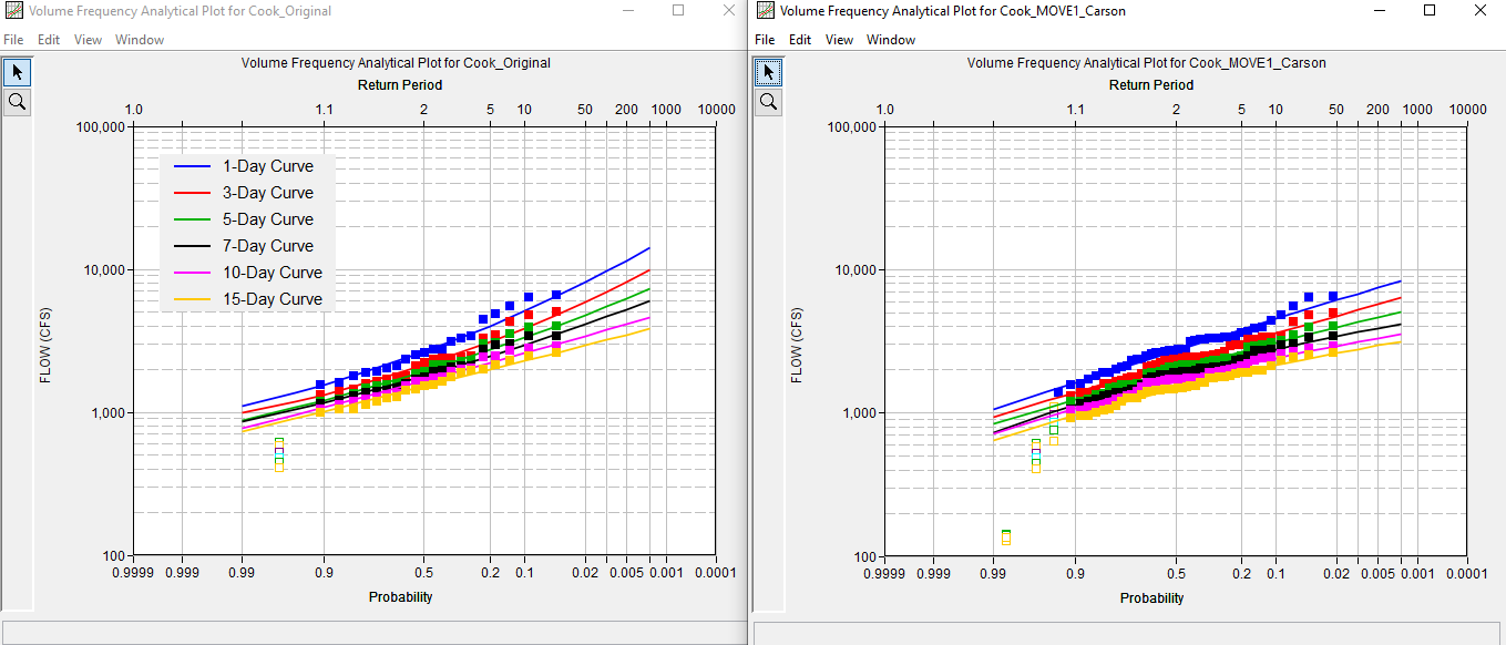
But is this really the best record extension? Probably not. While the MOVE.1 extension looked fairly reasonable for high flows, the MOVE.1 extension is greatly influenced by the low-flow data points. Since the regression is using every single day of daily data to come up with the MOVE.1 equation, the few high flow events have a relatively small influence on the record extension. If we really are interested in the 3-day flood volume frequency curve, the record extension should be tailored to high flow events and not unduly influenced by many days of low flows. 

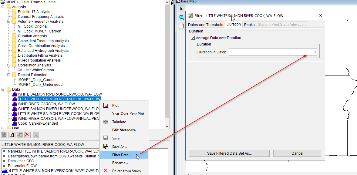
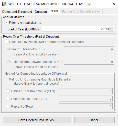
Often, an entire family of volume-frequency curves is not needed, and only a single duration is desired. If the 3-day volume frequency curve is the target, an alternate approach would be to perform a MOVE.3 analysis on the 3-day annual maximum volume time series. In SSP, create a 3-day annual maximum series by right clicking on the Cook dataset under the Data folder. Click Filter Data, and then calculate a 3-day average. Save this dataset. Right click the new dataset, and click Filter Data again. This time, select the Peaks tab, and then Filter to Annual Maxima. Change the start of the year to 01Oct (start of the water year). Save the annual maximum 3-day value. Repeat this process for the Carson gage.

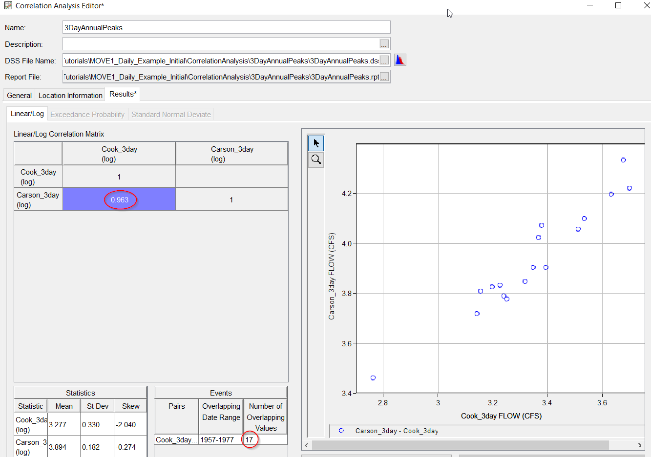
Check the data to make sure the 3-day peak at Cook occurs at roughly the same date as Carson. As shown previously in the tutorial: Using a Correlation Analysis to Select a Suitable Nearby Gage for Record Extension, a Correlation Analysis can be used for this purpose. The correlation of 0.963 is higher than the correlation between the daily average datasets. After inspecting the data, 17 of the 22 years of concurrent record had the 3-day maximum peak flow within a week. The remaining 4 events were not particularly notable, and the the MOVE.3 extension would likely be unaffected by correcting these points. These datasets were left as-is for this example. 

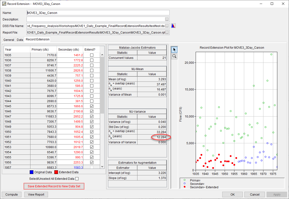
Perform a MOVE.3 extension of the Cook 3-day annual maximum volumes, using the Carson 3-day annual maximum volumes. Refer to the previous tutorial (Task 1. Create a new HEC-SSP Study and Import Data) for an example on how to do this. Note that the MOVE.3 extension only allows for 12 years of record to be added to avoid the long-term record at Carson from dominating the frequency curve calculation at Cook. Save the 3-day extended record to a new dataset. The 3-day extended record now spans from 1945-1977. 

Now, compute a Bulletin 17C analysis on the extended record. Refer to the previous tutorial (Annual Peak Flow Record Extension) for an example on how to do this.

At the 1% annual exceedance probability (100-year) event for the 3-day duration, the computed curve is 5815 cfs. This is lower than the original curve without record extension, and higher than the curve using MOVE.1 to extend daily flows back to 1935.

This example has shown 3 different methods of computing a 3-day volume frequency curve:

1. Original dataset only (1957-1977)
2. Daily average flow data extended with MOVE.1 (1935-1977)
3. 3-day annual maximum flow extended with MOVE.3 (1945-1977)

A comparison of the three methods of calculating the 3-day volume frequency curve is shown below. The uncertainty bounds on the calculated 3-day curve are also shown. Note that the uncertainty bounds using MOVE.3 are wider than calculated by MOVE.1, since the method does not attempt to extend the earlier years from 1935-1944. The MOVE.1 analysis includes these years and treats them as if they were the same quality as the original dataset, which artificially decreases the uncertainty in the curve. If there was no additional information available, the record extension with MOVE.3 on the 3-day volumes would be most appropriate.  

Download a copy of the final HEC-SSP project here - MOVE1_Daily_Example_Final.zip

FlowFrequencyCurve.xlsx