Download PDF
Download page Effective Record Length.
Effective Record Length
Overview
Previous versions of HEC-SSP reported inaccurate estimates of effective record length. These situations were most commonly encountered when large amounts of interval and/or censored data were incorporated within an analysis. The effective record length computations were improved within version 2.3 when using Bulletin 17C procedures to fit a LPIII distribution to annual maximum flow data.
This change only affects the reported effective record length. The parameterization of the distribution (i.e. mean, standard deviation, and skew), confidence limits, and quantile variance will be unaffected by these changes.
Background
A variety of stochastic (monte-carlo) based methods exist for the purpose of modeling uncertainty in an analytical flow-frequency curve. These models are commonly used to support a variety of risk-informed decisions. Some examples include the Watershed Analysis Tool (HEC-WAT), Flood Damage Reduction Analysis (HEC-FDA), Reservoir Frequency Analysis (RMC-RFA), and Stochastic Event Flood Model (SEFM). Effective record length (ERL) is commonly used as an input parameter to model the uncertainty in the flow-frequency curve using techniques such as the bootstrap (Efron, 1979) or parameter sampling distributions (USACE, 2016). ERL is synonymous with "equivalent record length".
ERL can be defined as “the number of years of systematic data that would produce the same MSE [or quantile variance] as a given combination of historical and systematic data” (Stedinger and Cohn, 1986). When all the input data are systematic (exact), ERL is simply equal to the record length. When some input data consists of flow interval, censored, or regional skew information, ERL is unknown and must be estimated. Cohn, Lane, and Baier (1997) proposed using Equation (1) to estimate effective record length after demonstrating that record length is asymptotically proportional to the inverse of quantile variance:
| 1) | E R L_p=N_S \frac{\operatorname{Var}\left[\hat{X}_p \mid N_S\right]}{\operatorname{Var}\left[\hat{X}_p \mid N_T\right]} |
where ERLp = effective record length at the pth quantile (years), p = a quantile where AEP = 1 - p, NS = number of systematic (exact) data, NT = number of combined systematic, historical, and censored data, Var[\hat{X}_{p}|N_{S}] = variance of the logarithm of flow at the pth quantile using only the systematic (exact) data, and Var[\hat{X}_{p}|N_{T}] = variance of the logarithm of flow at the pth quantile using the combined systematic, historical, censored, and regional skew information.
Improvements to ERL Computations
Three improvements to the ERL computations were made within HEC-SSP v2.3 when using Bulletin 17C procedures:
- The first improvement is to assume a linear relationship instead of a proportional relationship. This improves the accuracy of ERL estimates at record lengths on the order of 100 years or less.
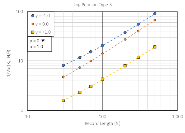
- The second improvement is to define quantile variance conditional on the parameter set for the combined systematic, historical, censored, and regional data. The linear (and proportional) relationships are only valid when the parameter set (i.e., the aleatory uncertainty) is held constant. Strictly speaking, only the standard deviation (σ) and skew (γ) parameters need to be held constant. Figure 1 shows the concept of a linear relationship conditional on a fixed parameter set where each parameter set corresponds to a unique line.

- The third improvement is to clarify that an average effective record length should be estimated for a set of quantiles specified by the user. The selected set of quantiles should reflect the range of primary importance for the stochastic analysis. Effective record length will be different at each quantile, but typical stochastic flood models require a single representative value.
These improvements were implemented using a standard linear interpolation formula like Equation (2) and then solving for the unknown ERLp. Specifically, HEC-SSP uses Equation (3) to estimate ERL:
| 2) | \frac{E R L_p-N_1}{\operatorname{Var}\left[\hat{X}_p \mid N_T, \theta_T\right]-\operatorname{Var}\left[\hat{X}_p \mid N_1, \theta_T\right]}=\frac{N_2-N_1}{\operatorname{Var}\left[\hat{X}_p \mid N_2, \theta_T\right]-\operatorname{Var}\left[\hat{X}_p \mid N_1, \theta_T\right]} |
| 3) | E R L_p=N_1+\left[\frac{\operatorname{Var}\left[\hat{X}_p \mid N_2, \theta_T\right]}{\operatorname{Var}\left[\hat{X}_p \mid N_T, \theta_T\right]}\right]\left[\frac{\operatorname{Var}\left[\hat{X}_p \mid N_1, \theta_T\right]-\operatorname{Var}\left[\hat{X}_p \mid N_T, \theta_T\right.}{\operatorname{Var}\left[\hat{X}_p \mid N_1, \theta_T\right]-\operatorname{Var}\left[\hat{X}_p \mid N_2, \theta_T\right]}\right]\left[N_2-N_1\right] |
where \operatorname{Var}\left[\hat{X}_p \mid N_2, \theta_T\right] = quantile variance for a hypothetical systematic dataset having a size of N2 and a parameter set of ΘT, \operatorname{Var}\left[\hat{X}_p \mid N_1, \theta_T\right] = quantile variance for a hypothetical systematic dataset having a size of N1 and a parameter set of ΘT, and ΘT = parameter set for the combined systematic, historical, and censored data. In theory, N1 and N2 can be assigned any arbitrary integer values so long as N1≠N2. In practice, values of N1=NS and N2=NT are a reasonable choice.
If N1 =N2, HEC-SSP will report an ERL = N1.
If NT > 500 (e.g., when paleoflood data is incorporate), HEC-SSP will set N2 = 500.
HEC-SSP will not extrapolate an ERL. If ERL > N2, HEC-SSP will report an ERL = N2.
Example Application for a Single Quantile
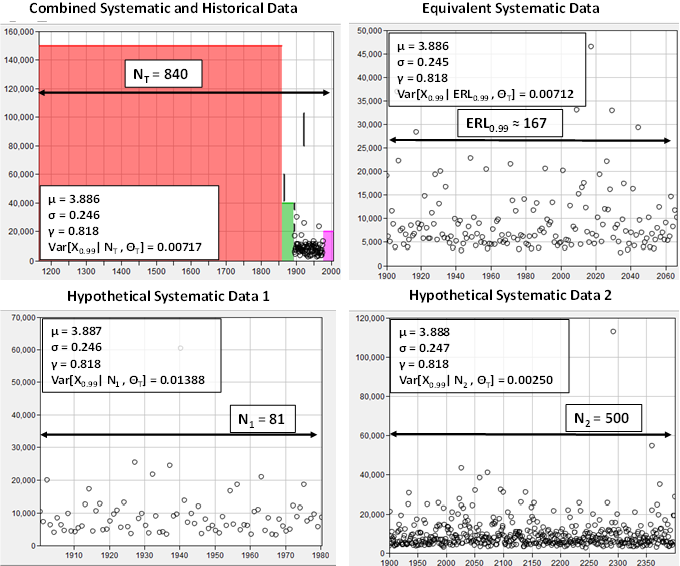
Figure 2 and Equation (4) summarize an example ERL calculation for a single quantile using Example 4 (Arkansas River at Pueblo, CO) presented in Appendix 10 of Bulletin 17C (England et al., 2019). The total record length of 840 years yields an ERL0.99 of approximately 167 years. Notice that the quantile variance for the combined dataset (Var[X0.99| NT , ΘT] = 0.00717) shown in the top left panel of Figure 2 is practically the same as the quantile variance for the equivalent systematic dataset (Var[X0.99| ERL0.99 , ΘT] = 0.00712) shown in the top right panel of Figure 2, thus satisfying the definition of ERL. For demonstration purposes, quantile variance for the two hypothetical systematic datasets shown in the bottom left and right panels of Figure 2 and the equivalent systematic dataset were estimated using HEC-SSP version 2.2 by generating synthetic systematic datasets having the specified record length and parameter set. Notice that the parameter sets \mu, \sigma, \gamma for all four datasets in Figure 2 are practically the same.
Within HEC-SSP v2.3, quantile variances are calculated using the specified record lengths and EMA-calculated parameter set without needing to generate synthetic datasets. This allows for a more direct and accurate estimation of ERL.

| 4) | E R L_0.99=81+\left[\frac{0.00250}{0.00717}\right]\left[\frac{0.01388-0.00717}{0.01388-0.00250}\right][500-81]=166 \text { years } |
Example Application for Multiple Quantiles
Within HEC-SSP v2.3, ERL is averaged for all quantiles less than or equal to 0.5 AEP in order to produce a best-estimate ERL for the entire distribution. ERL estimates for quantiles more frequently occurring than 0.5 AEP aren't incorporated in order to avoid complications arising from the presence of low outliers. Using the same example above, ERL for the quantiles of interest are shown in the table below.
| AEP | N1 Variance | N2 Variance | NT Variance | ERL (years) |
|---|---|---|---|---|
| 0.0001 | 0.084763 | 0.015494 | 0.049594 | 147.5 |
| 0.001 | 0.04049 | 0.007365 | 0.022431 | 156.0 |
| 0.002 | 0.030692 | 0.005568 | 0.016658 | 159.2 |
| 0.005 | 0.02012 | 0.00363 | 0.010614 | 163.6 |
| 0.01 | 0.013848 | 0.002482 | 0.007171 | 166.2 |
| 0.02 | 0.008984 | 0.001593 | 0.004628 | 166.0 |
| 0.05 | 0.004556 | 7.87E-04 | 0.002494 | 153.4 |
| 0.1 | 0.002556 | 4.27E-04 | 0.001655 | 126.8 |
| 0.2 | 0.001503 | 2.42E-04 | 0.001282 | 94.8 |
| 0.5 | 9.55E-04 | 1.57E-04 | 9.60E-04 | 80.5 |
The resultant averaged ERL is thus 141.4 years.