Download PDF
Download page Task 2 - Coincident Frequency by Monte Carlo Simulation.
Task 2 - Coincident Frequency by Monte Carlo Simulation
Task 2 is a continuation of the interior flooding analysis for Phillippi, West Virginia.
Until this point, we have assumed that interior precipitation is independent from exterior flow, meaning that these events are uncorrelated, and also don’t necessarily experience their annual peaks at the same time. Examine the two figures below to evaluate this assumption.


The figures above show Hall rainfall events and Tygart River high flow events plotted against each other. Correlation is demonstrated by values being large on both axes or small on both axes at the same time. Computed correlation is 41% for all rainfall events, and 35% for annual maxima rainfall events (paired with the streamflow that results). Generally, correlation greater than 30% between two variables is too high to ignore, so the assumption of no correlation, or independence, is not adequate here.
If we do not assume that the variables are independent, the correlation between variables could be captured by using a joint or conditional distribution of variable A. This characterization would require a family of frequency curves for Hall precipitation that are conditioned on Tygart River flow. While HEC-SSP has an option to use a conditional distribution of variable A on variable B, there is not usually enough data to develop such a distribution.
Correlation between the variables will instead be explored using a Monte Carlo simulation approach, using correlated sampling, performed in an MS Excel spreadsheet.
- From the Initial Workshop Files, open the spreadsheet named “coincident MC 2024.xlsm” (or, expand below to download).
- Hit the "Enable Content" button in the top yellow ribbon, if it appears.
- On the “variable A” tab, choose either GEV or Pearson3 (Pearson type III) from the dropdown, to match whichever distribution you chose in the General Frequency Analysis for Hall 3-day precipitation in HEC-SSP in Task 1.
- Next, copy in the distribution parameters – mean, standard deviation, and skew of the Pearson III distribution in cells E5:E7 or location, scale and shape of the GEV distribution in cells E30:E32.
- On the “variable B” tab, copy in the resulting daily duration curve from the Duration Analysis for Tygart streamflow in HEC-SSP in Task 1. Ensure the frequency ordinates (% of time exceeded) match between HEC-SSP and the spreadsheet. If the ordinates do not match, adjust them on the Duration Analysis Options tab and re-compute the results.
- The “response” tab already contains the response curves from the HEC-HMS runs. Note there are more rows and columns than used in HEC-SSP.
- The “sampling” tab performs the random sampling of 1000 pairs of an annual maximum 3-day precipitation at the Hall gage (variable A) along with a Tygart River daily flow value (variable B), with the correlation specified in cell G3. Leave correlation as 0 for now, and look at the plots of paired samples of N[0,1], U[0,1] and [precip, flow]. (The resulting sample correlation is in cell S9).
- Hit the F9 key several times to generate different samples of 1000 pairs.
- The “plot samples” tab shows the 1000-member samples of precipitation events and associated flow plotted with their input distributions.
- Hit the F9 key several times to generate samples of the 1000 pairs, while looking at the distribution plots.
- The “pond stage frequency” tab shows the resulting 1000 pond stages found by evaluating the 1000 pairs of precipitation and flow through the response curves. Values are sorted and plotted as a stage frequency curve in blue points, along with the HEC-SSP stage frequency curve in orange.
Hit the F9 key several times to see different samples of 1000 events.
Figures from "plot samples" tab:

Pond stage frequency with correlation = 0:
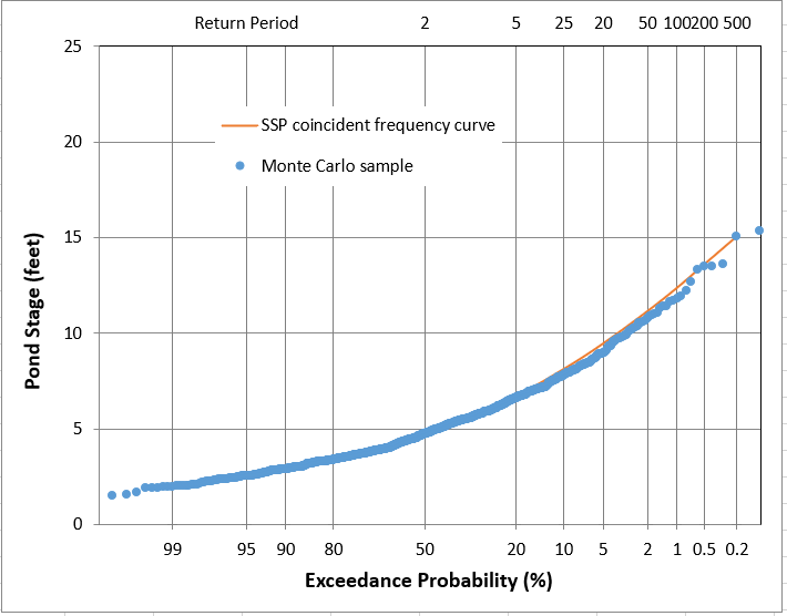

Question 1: Do you think 1000 events is a large enough sample for the MC analysis? Why or why not?
No, the fact that each sample shows a different resulting curve (especially at the top/right) shows that the sample is not large enough to have converged for extreme frequencies. NOTE: a new sample is generated with each press of the F9 key.
- Return to the “sampling” tab, and enter a correlation of 0.7 in cell G3. Note the images of the samples to see the correlation between the variables. Go to the “pond stage frequency” tab to see the resulting frequency curve.
- Hit the F9 key several times to see different samples of 1000 events.
Pond stage frequency with correlation = 0.7:
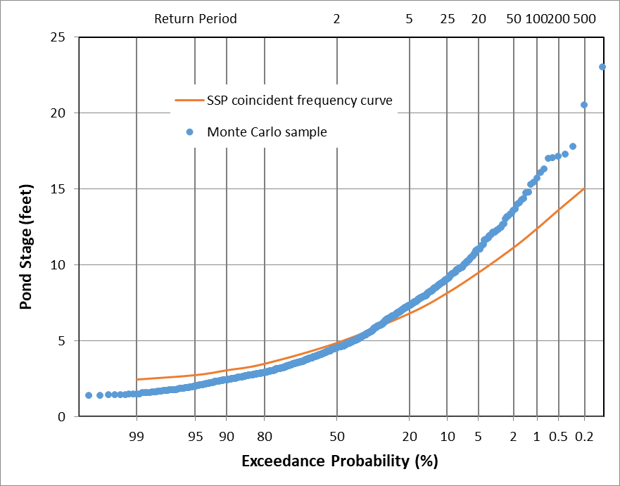
Question 2: What is the impact of considering correlation between the variables, compared to the original curve that is based on correlation=0?
When independence is not assumed and a positive (>0) correlation is used, the resulting frequency curve for pond stage is steeper (has a higher standard deviation), and is higher at the top (low frequencies) and lower at the bottom (high frequencies). Thus the curve shows more extremes than can occur without correlation.
Question 3: Why might this outcome be the case?
When 3-day max precipitation is correlated with streamflow, those values are more likely to be high at the same time, producing a higher pond stage. The independence assumption considers the 2 variables less likely to be high at the same time, producing lower pond stages in the upper tail. They are also less likely to be low at the same time, making the lower tail higher.
- Note correlation of 0.7 is higher than was estimated, and is used only to show the impact of correlation more clearly. Return to the “sampling” tab, and enter a correlation of 0.35 in cell G3. This value is closer to the estimated correlation between Hall 3-day precipitation and Tygart River flow.
Question 4: What is the outcome of performing an analysis that does not consider correlation?
The resulting frequency curve is lower (less conservative), and could under-predict the extreme events that will be experienced.
Final Workshop Files