Download PDF
Download page Task 4. Create Bulletin 17 Analyses for the 3-day Duration Inflow and Compute LPIII Parameters using Bulletin 17C Methodology.
Task 4. Create Bulletin 17 Analyses for the 3-day Duration Inflow and Compute LPIII Parameters using Bulletin 17C Methodology
In Tasks 1-3, you created a new HEC-SSP project, imported the necessary data sets, and extended the record using a nearby gage with additional information. In Task 4, you will create several Bulletin 17 analyses to fit LPIII analytical distributions to the 3-day duration inflow data sets using Bulletin 17C methodology.
The Bulletin 17C guidance incorporates changes motivated by more than 30 years of post-Bulletin 17B research on flood processes and statistical methods (England, et al., 2019). As part of the Bulletin 17C methodology, the moments/parameters of the LPIII distribution are estimated using the Expected Moments Algorithm (EMA). Like Bulletin 17B, the Bulletin 17C/EMA (17C EMA) methodology also estimates distribution parameters based on sample moments, but does so in a more integrated manner that incorporates non-standard, censored, or historical data at once, rather than as a series of adjustment procedures (Cohn, Lane, & Baier, 1997). The use of Bulletin 17C procedures also provides improved confidence intervals for the resulting frequency curve that incorporates skew uncertainty and diverse information appropriately, as historical data and censored values impact the uncertainty in the estimated frequency curve (Cohn, Lane, & Stedinger, 2001).
- Click Analysis | New | Bulletin 17 Analysis.
- Name the new analysis “3DAY_B17C”.
- Click the Flow Data Set drop down menu and select the original (i.e. unextended) data set (BALD EAGLE CREEK-SAYERS-FLOW-UNREG).
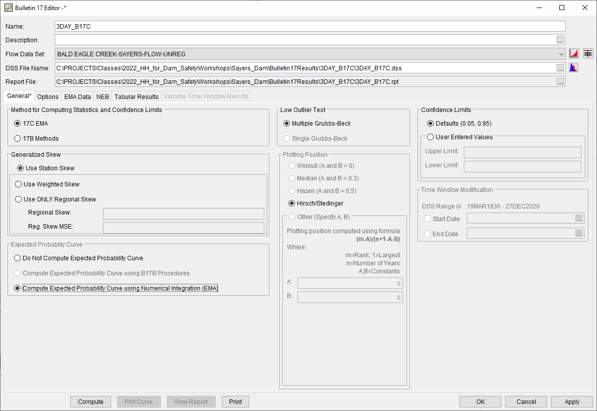
- Select “17C EMA” within the Method for Computing Statistics and Confidence Limits. This will automatically select other features including the Multiple Grubbs-Beck low outlier test and Hirsch/Stedinger plotting positions.
- Select the Compute Expected Probability Curve using Numerical Integration (EMA) radio button within the Expected Probability Curve panel.
- The General tab should look similar to the following figure.
- Move to the Options tab.
- Within the User Specified Frequency Ordinates section, click the Use Values from Table Below check box within the Output Frequency Ordinates panel.
- Right-click within the table and add an additional ten rows.
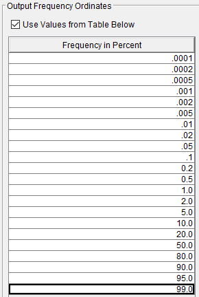
- Within the new rows, add the 0.0001-, 0.0002-, 0.0005-, 0.001-, 0.002-, 0.005-, 0.01-, 0.02-, 0.05-, and 0.1-percent frequency ordinates.
- This corresponds to the 1/1,000 to 1/1,000,000 annual exceedance probabilities (AEP).
- The Output Frequency Ordinates panel should look similar to the following figure.
- Move to the EMA Data tab.
The EMA procedure introduces the new concept of Perception Thresholds. Perception thresholds define the range of streamflow for which a flood event could have been observed. The inherent assumption and consequence is that any year for which an event was not observed and recorded must have had a peak flow rate outside of (usually below) the perception range.
The first row within the Perception Thresholds table will automatically be created to span the entire period of record of the selected Flow Data Set. The start and end year of this first perception threshold can be modified to alter the analysis time frame. This first perception threshold must have a low value of 0 and a high value of infinity. Additional rows within the perception threshold table supersede the rows above, for the specified time frame. Within HEC-SSP, perception threshold time frames should not overlap one another.
For any missing years in the analysis period, perception thresholds other than zero to infinity must be entered after the first row. The reason for this requirement is that a perception threshold of zero to infinity presumes any flow that occurred could have been observed, implying that unobserved years would not be possible. Therefore, unobserved years must have a perception threshold with either a lower bound greater than zero or an upper bound less than infinity. Most commonly, since very large flows tend to be observed in some way (as historical events are estimated based on some evidence in the watershed), a lower bound greater than zero is chosen.
Evidence presented in a March 1936 event post-flood report (Bogardus & Ryder, 1936) suggests that the March 1936 event was the largest peak flow rate in the Bald Eagle Creek watershed since at least 1911. This implies that had a flood larger than the March 1936 event occurred in the timeframe between 1911 and 1936, it would have been documented. Therefore, the analysis period can be extended to 1911.
- Change the first row in the Perception Thresholds table so that the analysis spans 1911 through 2021. The low and high perception thresholds for this first row should be left at 0 and “inf”.
- Perception thresholds other than zero to infinity must be added for the missing years in the analysis period. These missing years are 1911 – 1935 and 1937 - 1954. Therefore, two additional rows must be added to the Perception Thresholds table.
- Since the March 1936 event had a peak flow rate of approximately 9229 cfs, this flow rate can be used as a low threshold for the perception thresholds of those missing years.
Question 1: If a perception threshold of [9229 cfs – inf] is specified for 1937 – 1954, what is the complementary flow range for the same period?
The use of this perception threshold assumes that had a peak flow rate occurred in excess of 9229 cfs, it would have been documented. Therefore, the complementary flow range is [0 – 9229 cfs].
- In the second row of the Perception Thresholds table, type 1911, 1935, and 9229 in the cells corresponding to Start Year, End Year, and Low Threshold.
- Ensure that the High Threshold cell contains “inf”.
If it does not, double left-click within the cell to begin editing, right-click, and select Set as INF. This sets the high threshold to infinity.
- Use the Comments column to provide an adequate descriptive note.
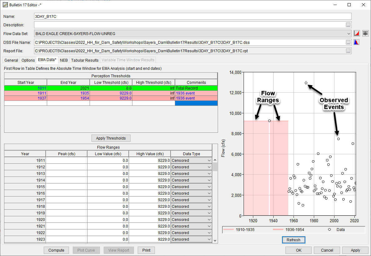
- Continue creating rows in the Perception Thresholds table until all of the missing years in the analysis period are accounted. The Perception Thresholds table should resemble the following figure.

- Once all of the information has been entered to the Perception Thresholds table, click Apply Thresholds. This will fill out the Flow Ranges table with the complementary information.
- Within the Flow Ranges table, change the Data Type for the 1936 event to Historical.
- Ensure that the Flow Ranges table contains a low and high value for every single year in the analysis period.
- The completed EMA Data tab should resemble the following figure.
- Click Compute.
- Click Plot Curve. This will result in the computed curve, expected probability curve, 5- and 95-percent confidence limits, and observed events being plotted.
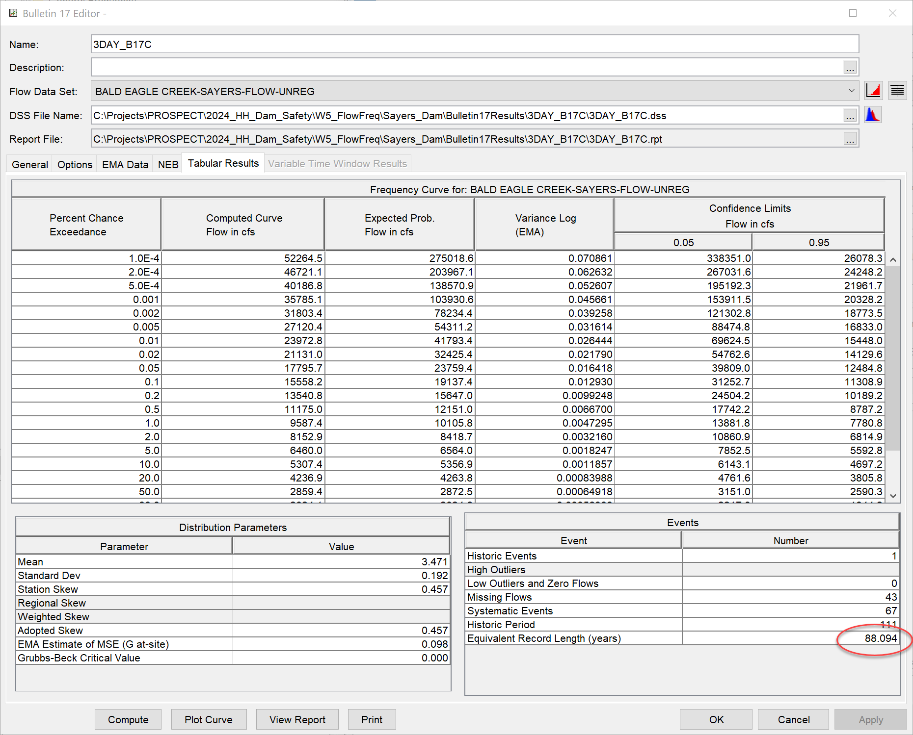
- Move to the Tabular Results tab. Note the computed curve, 5-, and 95-percent confidence limits for all of the desired frequency ordinates, the moments/parameters of the LPIII distribution fit to the data, and other data related to the analysis are shown.
Question 2: What is the Equivalent Record Length (ERL) for the 3DAY_B17C analysis?
Effective record length (ERL) can be defined as “the number of years of systematic data that would produce the same mean square error [or quantile variance] as a given combination of historical and systematic data” (Cohn and Stedinger, 1986). When all the input data are systematic (i.e. exact), ERL is simply equal to the record length. When some input data consists of flow interval, censored, or regional skew information, ERL is unknown and must be estimated. A variety of stochastic (Monte Carlo) based methods exist for the purpose of modeling uncertainty in an analytical flow-frequency curve. These models are commonly used to support a variety of risk-informed decisions. Some examples include the Watershed Analysis Tool (HEC-WAT), Flood Damage Reduction Analysis (HEC-FDA), and Reservoir Frequency Analysis (RMC-RFA). ERL is commonly used as an input parameter to model the uncertainty in the flow-frequency curve using techniques such as the bootstrap (Efron, 1979) or parameter sampling distributions (USACE, 2016).
The ERL for this analysis is approximately 88 years. This information can be found on the Tabular Results tab, as shown in the following figure.
Next, create a Bulletin 17 analysis and fit an LPIII analytical distribution to the extended 3-day duration inflow data set using Bulletin 17C methodology.
- Right click on the existing "3DAY_B17C" analysis and select Save As.
- Name the new analysis “3DAY_Extended_B17C”.
- Open the new analysis, click the Flow Data Set drop down menu, and select the extended data set (SayersDam_3day_MOVE3).
- Move to the EMA Data tab.
- Double left click in the upper-left cell in the Perception Thresholds table and hit enter.
This applies the extended analysis window to the Flow Ranges table below.
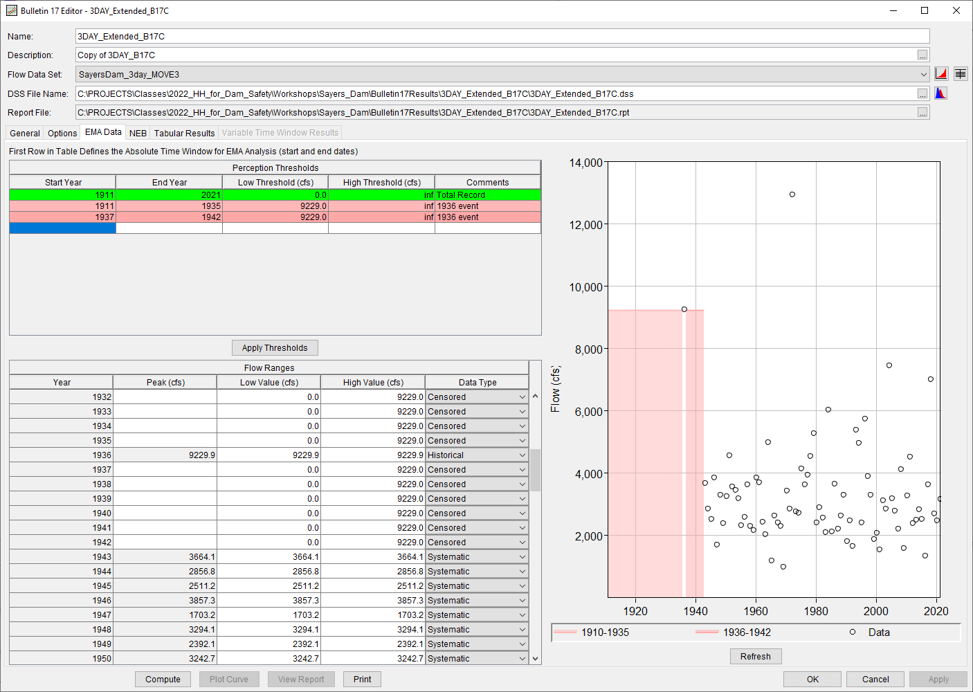
- Since the extended data set contains additional years of record, change the third row in the Perception Thresholds table to span 1937 through 1942. The low and high perception thresholds for this first row should be left at 9229 and “inf”.
- Once all of the information has been entered to the Perception Thresholds table, click Apply Thresholds. This will fill out the Flow Ranges table with the complementary information.
- Within the Flow Ranges table, change the Data Type for the 1936 event to Historical.
- Ensure that the Flow Ranges table contains a low and high value for every single year in the analysis period.
- The completed EMA Data tab should resemble the following figure.
- Click Compute.
- Click Plot Curve. This will result in the computed curve, expected probability curve, 5- and 95-percent confidence limits, and observed events being plotted.
- Move to the Tabular Results tab. Note the computed curve, 5-, and 95-percent confidence limits for all of the desired frequency ordinates, the moments/parameters of the LPIII distribution fit to the data, and other data related to the analysis are shown.
The 3DAY_B17C and 3DAY_Extended_B17C results can be plotted at the same time by selecting both analyses in the main HEC-SSP window and clicking Results | Graph.
Question 3: How different are the 3DAY_B17C and 3DAY_Extended_B17C results? Compare the various outputs at multiple annual exceedance probabilities (AEP).
The 3DAY_B17C analysis resulted in an LPIII with a smaller mean, larger standard deviation, and larger skew than the 3DAY_Extended_B17C analysis. The 3DAY_B17C results (red curves) plot to the left/above the 3DAY_Extended_B17C results (green curves), as shown in the following figure.
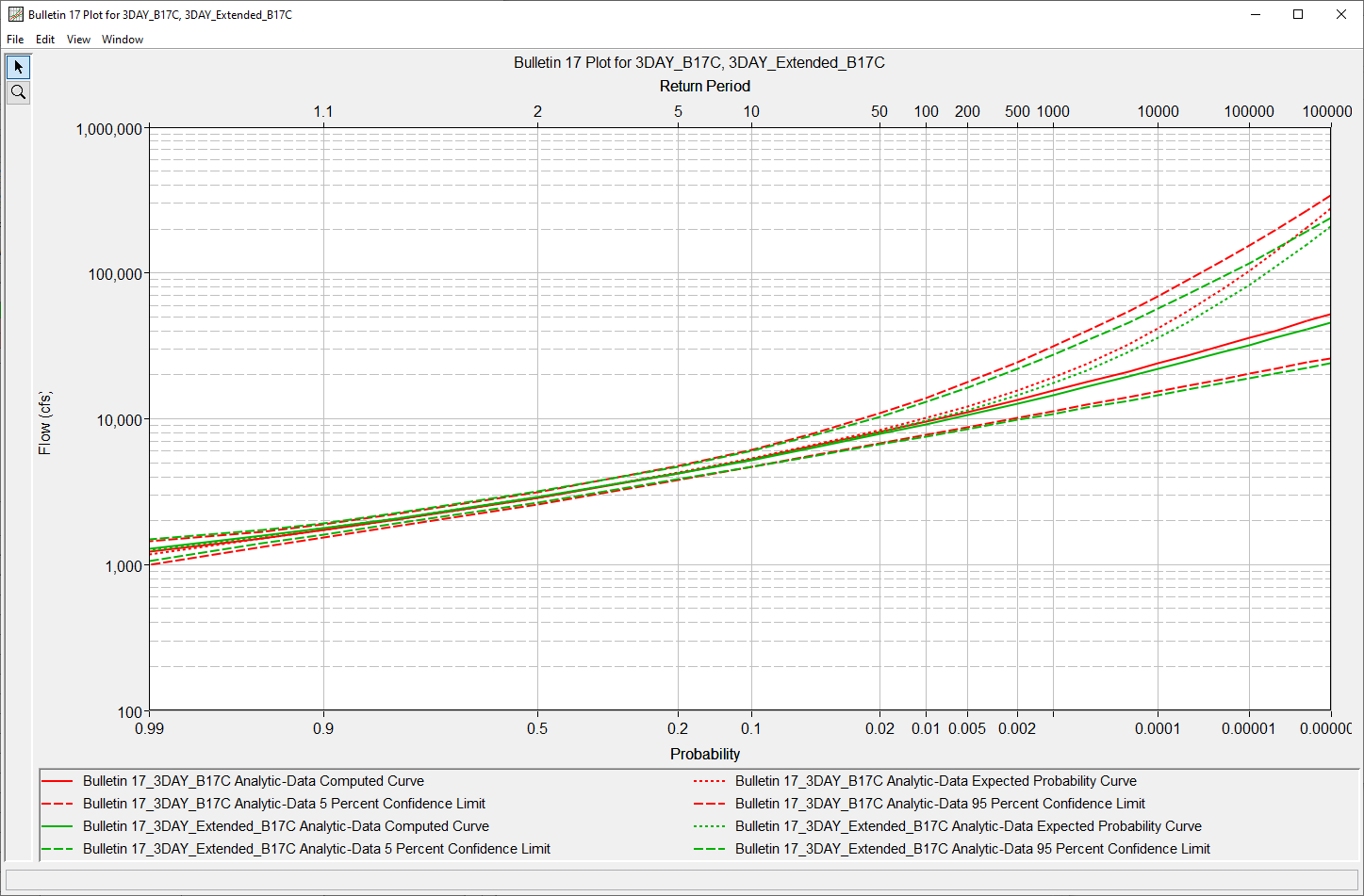
For extremely large flow rates (e.g. 100,000 cfs), the predicted AEP is approximately 1/4 order of magnitude rarer in probability space. This indicates that the extended record resulted in smaller predicted flow rates for rare AEP.
Question 4: What is the ERL for the 3DAY_Extended_B17C analysis? How much additional information content was added by including the extended record?
The ERL for this analysis is approximately 94 years. This indicates that the MOVE.3 record extension added approximately 6 years' worth of information content when compared against the 3DAY_B17C analysis.
Download the final project files here: Sayers_Dam.zip
Continue to Task 5. Incorporate Paleoflood Information, Compute New LPIII Parameters, and Compare the Results.