Download PDF
Download page Optional Task. Analyze the East Fork Big Creek Data Set Using B17B Methods.
Optional Task. Analyze the East Fork Big Creek Data Set Using B17B Methods
Return to Optional Task. Analyze the Santa Cruz River Data Set using B17B Methods.
Create a New Bulletin 17 Analysis
- Create a Bulletin 17 analysis.
- Go to the Analysis menu and select New | Bulletin 17 Flow Frequency to open the Bulletin 17 editor.
- Enter a name to describe the analysis like “East_Fork_Big_Creek”.
- Select the Flow Data Set labeled “East Fork Big Creek-Bethany, MO-FLOW-ANNUAL PEAK”.
- Select the 17B Methods radio button.
- Ensure the following options are selected:
- Use Station Skew.
- Select the Do Not Compute Expected Probability Curve
- Select the Single Grubbs-Beck
- Select the Median plotting position formula.
- Press the Compute button..
Analyze Results
- Navigate to the Tabular Results tab.
- Graph the results by selecting the Plot Curve.
- Click the Save button (
 ) to save the study.
Question: Comment on the fit of the frequency curve to the data and its reasonableness. Are there any high and low outliers?
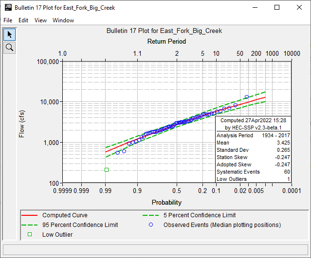
There is one low outlier and no high outliers when using the default outlier thresholds, as shown in the following figure. The highest and lowest points seem somewhat inconsistent with the curve. The curve’s estimated exceedance probability for the 1973 event is beyond 0.2% (i.e. 1/500 annual chance exceedance).

Add a Historical Event
- Create a copy of the East Fork Big Creek Bulletin 17 analysis and add the historical event.
- Place the mouse pointer on top of the existing East_Fork_Big_Creek Bulletin 17 analysis and click the right mouse button. Select the Save As… option in the pop-up menu.
- Enter a Name for the new Bulletin 17 analysis, “East_Fork_Big_Creek_Hist” and click the OK The new Bulletin 17 analysis will be added to the study.
- Open the copied Bulletin 17 analysis and select the Options tab.
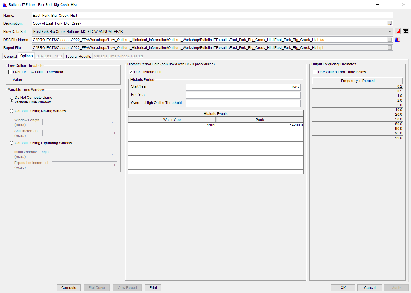
- Check the box to Use Historic Data. Enter a Start Year of 1909.
- In the Historic Events table, add 1909 and an estimate flow of 14,200 cfs, as shown in the following figure.

- Compute the analysis and plot the frequency curve.
- To see the impact of using the historical event, select both analyses (with and without the historical event) in the study tree and plot the curves together.
Question: How did the use of an historical event affect the frequency curve?
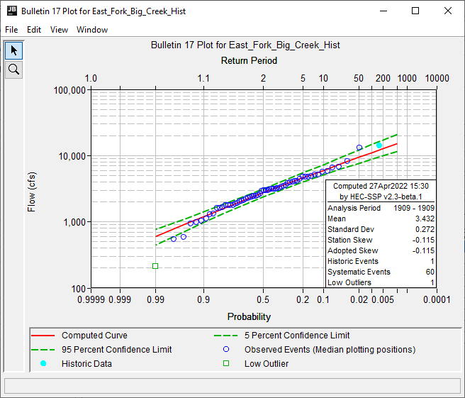
As shown in the following figure, the upper end of the frequency curve was raised when the historical 1909 event was added. Because the plotting positions changed with the inclusion of historical information, adding the historical event makes the large 1973 event seem more likely, which is perhaps not correct. However, the frequency curve’s estimate of the exceedance probability of the 1973 event is about 0.4% (i.e. 1/250 ACE).

Add a Second Historical Event
Consider the events in the period of record. Note the 1973 event is significantly larger than the rest of the systematic events, and nearly as large as the 1909 event. The USGS code for 1973 designates it as an historical event as well. A high outlier threshold should be specified so that this event is treated as an historical event.
- Create a copy of the East_Fork_Big_Creek_Hist Bulletin 17 analysis and add a high outlier threshold that is less than the 1973 event.
- Use the Save As option. Name the new Bulletin 17 analysis “East_Fork_Big_Creek_HistHi”.
- On the Options tab, enter a value less than the magnitude of the 1973 event within the Override High Outlier Threshold entry field, as shown in the following figure.

- Compute the analysis and plot the frequency curve.
- To see the impact of making 1973 a high outlier, select both analyses in the study tree and plot the curves together.
Question: How did making 1973 a high outlier (historical event) affect the frequency curve?
The top end of the frequency curve is lower when 1973 becomes a historical event. This effect is due to the same logic as moving the 1973 point to the right, with a smaller exceedance probability. Note, this change seems to undo the effect of adding the historical value. The curve with both the historical event and the high outlier is very similar to the curve from only the systematic data.
Question: Consider the LPIII frequency curve and all the plotted data. How many low outliers are censored by the default low outlier threshold? Do the remaining low events seem influential?
Only 1 low outlier has been censored. It would be reasonable to censor 2 more, to see if they are decreasing the skew and pulling the upper end of the curve down more than the higher data suggests. Censoring the 2 more low outliers raises the upper end of the frequency curve and makes it more consistent with the higher points.
- Create a copy of the East_Fork_Big_Creek_HistHi Bulletin 17 analysis and override the low outlier threshold:
- Place the mouse pointer on top of the existing East_Fork_Big_Creek_HistHi Bulletin 17 analysis and click the right mouse button. Select the Save As… option in the pop-up menu.
- Enter a Name for the new Bulletin 17 analysis, “East_Fork_Big_Creek_HistHiLow” and click the OK The new Bulletin 17 analysis will be added to the study.
- Open the copied Bulletin 17 analysis and select the Options Check the box to Override the Low Outlier Threshold and then enter a value. Choose a value that you feel improves the frequency curve fit to the data.
- Compute the analysis and Plot the frequency curve.
Question: Compare the three frequency curves: the first estimate, HistHi, and HistHiLow. How does adding the historical event, overriding the high outlier threshold, and overriding the low outlier threshold affect the frequency curve?
Adding the historical event and specifying 1973 as a high outlier ends up changing the frequency curve very little. However, the specification of 3 rather than 1 low outlier raises the upper end of the curve in a way that is more consistent with the higher data.
Question: How comfortable do you feel (arbitrarily) changing the number of values that are considered high outliers, historical events, and/or low outliers?
If you're like me, you feel very uncomfortable doing this. This question is meant to incite discussion and promote the use of Bulletin 17C procedures.
Question: Compare the flow-frequency curve developed using Bulletin 17C and those develop using Bulletin 17B procedures (use the analysis that includes 1909 but no low outlier overrides). How do these curves contrast one another? If time allows, explore the use of other perception thresholds that can be justified and note the effect on the LPIII distribution/curve.
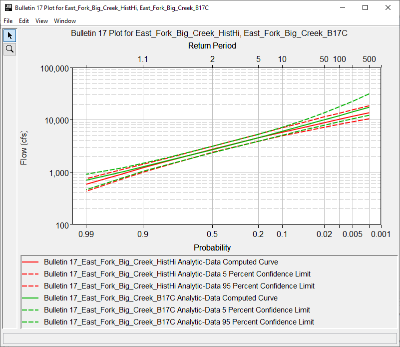
The Bulletin 17C curve exhibits a slightly positive skew while the Bulletin 17B curve exhibits a slightly negative skew. This results in relatively large differences in flow values for rare exceedance probabilities (i.e. 1/500), as shown in the following figure. Also, the confidence intervals for the Bulletin 17C compute are wider than those computed using Bulletin 17B techniques.

Continue to Optional Task. Compare B17B and B17C Low Outlier Procedures.