Optional Task. Analyze the Santa Cruz River Data Set using B17B Methods

Continue by using the project from Task 3. Analyze the East Fork Big Creek Data Set Using B17C Methods.

Create a New Bulletin 17 Analysis

Create a flow frequency analysis using Bulletin 17B procedures. Go to the Analysis menu and select New | Bulletin 17 Flow Frequency to open the Bulletin 17 editor.
Enter a name to describe the analysis like “Santa_Cruz_River”.
Select the Flow Data Set labeled “SANTA CRUZ RIVER-LOCHIEL, AZ-FLOW-ANNUAL PEAK”.
Select the 17B Methods radio button.
Ensure the following options are selected:
- Use Station Skew.
- Select the Do Not Compute Expected Probability Curve.
- Select the Single Grubbs-Beck.
- Select the Median plotting position formula.
Press the Compute button.

Analyze Results

Navigate to the Tabular Results tab.
Graph the results by selecting the Plot Curve button.
Note the Log Pearson III statistics and the number of high and low outliers.
Plot the curve using the Plot Curve button, and examine the fitted curve and the low outliers.

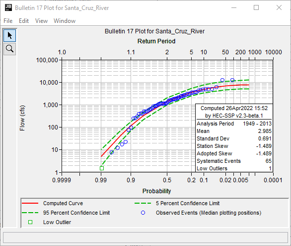
Question: Comment on the fit of the frequency curve to the data and its reasonableness. How would the fitted curve estimate the exceedance probability of the largest 2 events? Discuss what might be influencing the fit.

The computed skew is -1.498, which is VERY negative . The upper end of the frequency curve reaches an upper bound at about 8,000 cfs due to this skew, as shown in the figure below. The two highest events in the record are greater than 8,000 cfs, which is clearly inconsistent with this estimated curve. It seems the frequency curve is getting a very negative skew due to the low values. There was 1 low outlier identified. Given the break from the rest of the systematic data, more low outliers could reasonably be censored.

Override the Low Outlier Threshold

Create a copy of the Santa_Cruz_River Bulletin 17 analysis and override the low outlier threshold. Place the mouse pointer on top of the existing Santa_Cruz_River Bulletin 17 analysis and click the right mouse button. Select the Save As… option in the pop-up menu.
Enter a Name for the new Bulletin 17 analysis, “Santa_Cruz_River_low” and click the OK. The new Bulletin 17 analysis will be added to the study.
Open the copied Bulletin 17 analysis and select the Options Check the box to Override the Low Outlier Threshold and then enter a value.

Choose a low outlier threshold that you think improves the frequency curve fit to the data. Try multiple low outlier thresholds.

Compute the analysis and plot the frequency curve.
Compare the frequency curve to the original frequency curve computed using the default low outlier threshold.
- Select both Bulletin 17 analyses and click Results | Graph.
Continue exploring the impact of various low outlier thresholds until you feel you have a final selection. Consider using Save As… feature to compare multiple threshold choices by selecting multiple analyses in the study tree and choosing Results | Graph.

Question: Discuss the impact of the low outlier thresholds you evaluated. Which value provides the best fit? How does this impact the upper end of the curve (i.e. for smaller exceedance probabilities)?

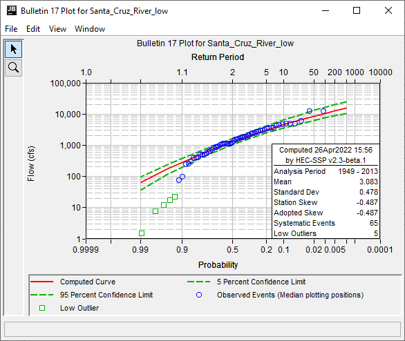
Putting the low outlier threshold at 30 cfs censors a total of 5 low outliers. The skew is raised to -0.487, and the upper end of the curve is more consistent with the highest points. The following figure shows the curve with 5 low outliers censored. If the low outlier threshold is raised to 100 cfs, a total of 7 low outliers are censored. It is subjective, at best, to say which frequency curve is most reasonable.

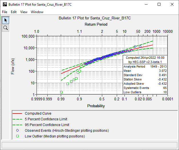
Question: Compare the flow-frequency curves created using the Bulletin 17B techniques (without and with your defined low outlier threshold) and the flow-frequency curve created using Bulletin 17C techniques. Discuss the result of the Multiple Grubbs-Beck test. Compare the B17C curve to the various B17B curves. Compare the confidence intervals of the B17C curve to the B17B curves. Which method produces a more reasonable estimate of annual chance exceedance for the most extreme observed events? (Hint: this is a subjective question and meant to incite discussion).

The MGB test found 10 low outliers, or more specifically, PILFs, as shown in the following figure. The upper end of the curve seems consistent with the plotted points. The upper end is also between the 5-low-outlier and 7-low-outlier options from the B17B computes, but the lower end is more consistent with the low data. The confidence limits for the B17C curve are notably wider than the confidence limits for the B17B curves. This is because of the more correct incorporation of skew uncertainty into the confidence limits.

Continue to Optional Task. Analyze the East Fork Big Creek Data Set Using B17B Methods.