Download PDF
Download page Task 2. Analyze the Santa Cruz River Data Set Using B17C Methods.
Task 2. Analyze the Santa Cruz River Data Set Using B17C Methods
Return to Task 1. Create a New Project and Import Data.
Analyze the Santa Cruz River Data Set
Prior to fitting any analytical distributions, it's recommended to first inspect the data set.
Question: How many annual peaks are contained within the Santa Cruz River data set?
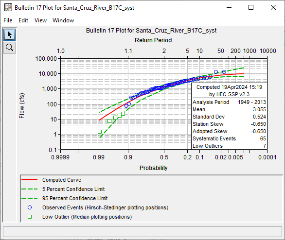
This data set consists of 65 annual maxima beginning in water year 1949 and ending in water year 2013.
Question: What are the magnitudes of the two largest flood events within this data set?
A large flood event occurred on October 9, 1977 with a magnitude of 12000 cfs. The August 15, 1984 flood magnitude is equivalent to the October 1977 flood peak.
Create a New Bulletin 17 Analysis for the Systematic Data
- Create a flow frequency analysis using Bulletin 17C procedures. Go to the Analysis menu and select New | Bulletin 17 Flow Frequency to open the Bulletin 17 editor.
- Enter a name to describe the analysis like “Santa_Cruz_River_B17C_Syst”.
- Select the Flow Data Set labeled “SANTA CRUZ RIVER-LOCHIEL, AZ-FLOW-ANNUAL PEAK”.
- Select the 17C EMA radio button.
- Ensure the following options are selected:
- Use Station Skew.
- Select the Multiple Grubbs-Beck
- Select the Hirsch/Stedinger plotting position formula.
Review EMA Data for the Systematic Period
- Move to the EMA Data.
- Ensure that the Flow Ranges table is completely filled out and all years use the Systematic data type.
- No additional modifications are necessary for the systematic period.
Compute and Analyze the Systematic Period Results
- Press the Compute button.
- View the Tabular Results tab, and note the LogPearsonIII statistics and the number of low outliers/PILFs.
- Plot the flow-frequency curve using the Plot Curve button and examine the fitted curve and the low outliers.
- Click the Save button (
 ) to save the study.
Question: How many low outliers/PILFs were identified within the systematic analysis?
Ten low outliers/PILFs were identified, as shown below.

Question: What changes were automatically made to the perception thresholds and flow ranges for each systematic event?
Detailed diagnostic data can be found within the Report file, which can be opened by clicking the View Report button.
The MGB test identified a low outlier threshold (critical value) of 380 cfs, which corresponds to the smallest peak that was retained. The perception threshold for all systematic observations was adjusted to [380 cfs – inf]. Additionally, the flow range for each of the ten annual peaks that were less than the MGB critical value was recoded to span [0 - 380 cfs]. The flow range for events that were greater than or equal to the MGB critical value were left as-is, as shown in the Report file.

Now, investigate the sensitivity of the results when using different MGB threshold values.
- Navigate to the Options tab.
- Enable the Override Low Outlier Threshold option by clicking the checkbox.
- Try entering different values in this entry field, recompute, and note the differences.
Question: How many events are censored when using a threshold of 243 cfs? How many events are censored when using a threshold of 73 cfs? Do these threshold values produce acceptable answers?
This question is meant to incite discussion.
The largest three events that were censored aren't plainly evident to be different than annual maxima that weren't censored. Overriding the low outlier threshold on the Options tab, entering a value of 243 cfs (to censor three fewer values than the default MGB threshold), and recomputing results in flow frequency estimates that are similar to using the default MGB threshold.
However, censoring 2 fewer values by using a threshold of 73 cfs produces flow frequency estimates that are non-sensical. For instance, the two largest observed systematic events are predicted to have AEP of ~0.
- Turn off the Override Low Outlier Threshold option to return to using the default MGB threshold and recompute the analysis.
Create a New Bulletin 17 Analysis to Incorporate Historical Data
- Create a flow frequency analysis by selecting New | Bulletin 17 Flow Frequency to open the Bulletin 17 editor.
- Enter a name to describe the analysis like “Santa_Cruz_River_B17C_systHist”.
- Select the Flow Data Set labeled “SANTA CRUZ RIVER-LOCHIEL, AZ-FLOW-ANNUAL PEAK”.
- Select the 17C EMA radio button.
- Ensure the following options are selected:
- Use Station Skew.
- Select the Multiple Grubbs-Beck
- Select the Hirsch/Stedinger plotting position formula.
Add EMA Data for the Historical Period
- Move to the EMA Data.
Historical information indicates that the October 1977 flood event was the largest since at least 1927 (Aldridge & Eychaner, 1984). This information can be used to extend the historical period through the use of a perception threshold.
- Change the first row of the Perception Thresholds table so that the analysis spans 1927 through 2013. The low and high perception thresholds for this first row should be left at 0 and “inf”.
- Add a second perception threshold of [12000 - inf] for the period of missing data spanning water years 1927 through 1948.
- Use the Comments column to provide an adequate descriptive note for the new row.
- Click the Apply Thresholds button to assign the complementary flow ranges for the periods of missing data.
- Ensure that the Flow Ranges table contains a low and high value for every single year in the analysis period.
- The completed EMA Data tab should resemble the following figure.

Compute and Analyze the Historical Period Results
- Press the Compute button.
- View the Tabular Results tab, and note the LogPearsonIII statistics and the number of low outliers/PILFs.
- Compare the results of the systematic-only and systematic + historical analyses.
- Click the Save button () to save the study.
Question: What changes were automatically made to the perception thresholds and flow ranges for each year in the historical period?
The perception threshold for the years in which there is only historical nonexceedance data (i.e. 1927 – 1948) were left at 12,000 - inf. Also, the flow range for these years was left unchanged and corresponds to the complementary flow range from the perception theshold.
Question: How did the inclusion of additional historical information affect the Log Pearson Type III parameters (mean, standard deviation, and skew)? How does this affect the computed flow-frequency information?
The mean, standard deviation, and skew magnitudes for the systematic + historical analysis are slightly less than the systematic-only analysis. This translates into slight decreases in quantile estimates (i.e., flow for a given probability). The ERL for the systematic + historical analysis is approximately 85 years. This translates into tighter confidence limits and less uncertainty in the computed flow-frequency information.
Continue to Task 3. Analyze the East Fork Big Creek Data Set Using B17C Methods.