Download PDF
Download page Task 3. Analyze the East Fork Big Creek Data Set Using B17C Methods.
Task 3. Analyze the East Fork Big Creek Data Set Using B17C Methods
Return to Task 2. Analyze the Santa Cruz River Data Set Using B17C Methods.
Analyze the East Fork Big Creek Data
Prior to fitting an analytical distribution, it's recommended to first inspect the data set.
Question: How many annual peaks are contained within the East Fork Big Creek data set?
This data set consists of 60 annual maxima beginning in water year 1934 and ending in water year 2017.
Question: How many missing periods of record are present within the systematic record?
Two missing periods spanning 1) 1973 - 1996 and 2) 2000 are present within this data set.
Check USGS Peak Flow Codes
USGS publishes codes that provides descriptive information about the peak flow estimates for each year. When data is imported into HEC-SSP from the USGS, these peak flow codes are also imported.
- Select both the East Fork Big Creek flows and codes.
- Plot and/or tabulate the data sets by clicking Data | Plot. The plot should resemble the following figure:

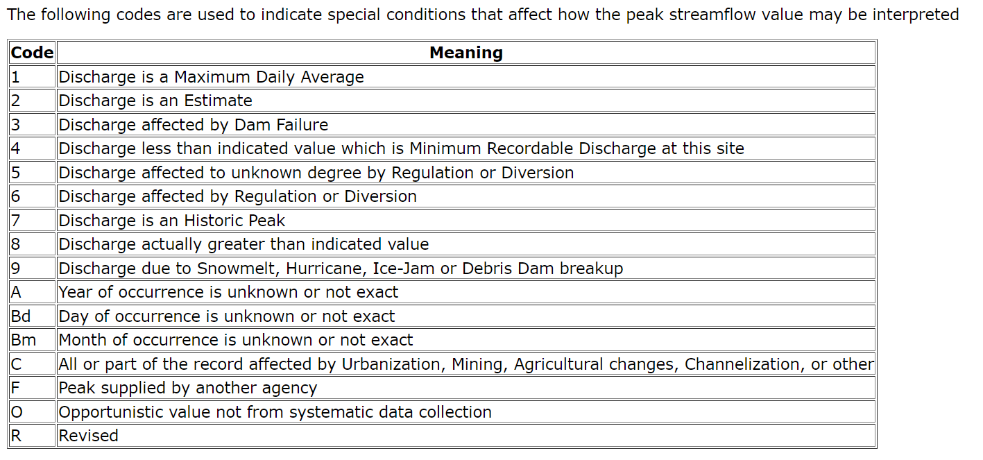
Question: Using the USGS code interpretations shown above, should the 13 October 1973 (Water Year, WY 1974) peak be represented using a Systematic data type? Where will this data need to be entered within the Bulletin 17 analysis?
No. The 13 October 1973 (WY1974) peak should be represented using a Historical data type due to the presence of a Code 7. This distinction will need to be made on the EMA Data tab.
Estimate a Peak Flow For WY1909
- Investigating the East Fork Big Creek NWIS Data shows that a measured peak stage (23.8 ft) is available for WY1909, but no corresponding peak flow is available, as shown in the following figure.

- An estimate of the peak flow for WY1909 can be by developing flow vs. stage relationships using data from 1934 – 1955 and 1956 – current.
- The data was split because the flow/stage relationship noticeably differed between the earlier period and the later period, as can be seen in the following figure.
")
Using these stage-flow rating curves, the peak flow for the 1909 event was estimated as 14,200 cfs.
Create a New Bulletin 17 Analysis
- Go to the Analysis menu and select New | Bulletin 17 Flow Frequency to open the Bulletin 17 editor.
- Enter a name to describe the analysis like “East_Fork_Big_Creek_B17C”.
- Select the Flow Data Set labeled “East Fork Big Creek-Bethany, MO-FLOW-ANNUAL PEAK”.
- Select the 17C EMA radio button.
- Ensure the following options are selected:
- Use Station Skew.
- Select the “Do Not Compute Expected Probability Curve” option.
- Select the Multiple Grubbs-Beck
- Select the Hirsch/Stedinger plotting position formula.
Input EMA Data
- Move to the EMA Data tab.
- By default, the Perception Threshold table should have a row for 1934 – 2017 and a perception threshold of [0 – inf].
- Within the Perception Thresholds table, change the Start Year of the first row to 1909.
- Click the Apply Thresholds button.
- Notice that the Flow Ranges table now has rows for 1909 – 1933 with no information.
Question: Non zero to infinity perception thresholds must be set for all missing years (1909 - 1933, 1973, 1975 - 1996, and 2000). What are reasonable values for the low threshold for each period?
As a start, for the missing historical years prior to 1934, we can assume they do not exceed the 1909 event, or there would have been some evidence found and noted. For the missing years in the record, we can conservatively say they did not exceed the 1974 values of 13000, or likewise would have been noted. To assume we truly know nothing about those years, we would use bounds [inf – inf], which implies a flow range of [0 – inf].
- Within the Flow Ranges table, add a value of 14200 cfs for 1909. Ensure the Low and High values are also set to 14200 cfs for this year as well.
- Change the data type for the 1909 and 1974 events to Historical.
- Add a row to the Perception Thresholds table from 1909 – 1933 and specify a reasonable low perception value. Make sure the high value is set to “inf” (infinity).
To enter “inf” within a cell, begin editing the cell by double left clicking, then right click, and select “set as INF”.
- Add rows to the Perception Thresholds table for the missing years in the record (i.e. 1973, 1975 - 1996, 2000). The Perception Thresholds table should resemble the following figure.

- When the perception thresholds table is complete, press the Apply Thresholds button. Complementary flow ranges inferred from the perception thresholds will be added to the Flow Ranges table. Check all years for both the flow values and data types.
Note: missing years should be set to Censored.
- The EMA Data tab should resemble the following figure.

Compute and Analyze Results
- Press the Compute button.
- Once the compute finishes, examine the Tabular Results tab, Plot the curve, and review the Report.
Question: How many low outliers (PILFs) were found? Do these values make sense?
Seven PILFs were identified using the MGB test. When viewing the flow-frequency curve and plotting positions for the observe data on a normal probability scale, it is evident that the three smallest annual peaks are markedly different than the remainder of the data. However, the four remaining censored events aren't drastically different than the rest of the sample.
- Override the low outlier threshold on the Options tab to use a threshold that will censor the 3 smallest events and note the results.
- Override the low outlier threshold on the Options tab to use a threshold that will censor a total of 9 events and note the results.
Question: How do these changes in the Low Outlier Threshold affect the results?
An override of 925 cfs should be used to censor the 3 smallest events. This change results in minor differences to the computed results when compared to the default MGB critical value.
An override of 1610 cfs should be used to censor the 9 smallest events. This change results in noticeable differences to the computed results when compared to the default MGB critical value. Specifically, the skew becomes positive and quantile estimates for rare AEP (e.g., 1/100) increase by approximately 1000 cfs.
- Turn of the Override Low Outlier Threshold on the Options tab to use the default MGB critical value.
- On the EMA Data tab, set the WY1974 peak to use a Systematic data type and recompute.
Question: How does treating the WY1974 peak as a Systematic Event affect the results?
When the WY1974 peak is set to use a Systematic data type, only 3 low outliers are identified by the MGB test. However, this results in only minor changes to the parameterized distribution and quantile estimates. This change occurs due to the fact that when an event is set to use a Historical data type, it is excluded from consideration within the MGB test. While there were little to no changes in the quantile estimates due to this change, it does highlight the sensitive nature of the MGB test when it comes to the treatment of data.
Conclusion
This concludes the Frequency Curves with Low Outlier and Historical Information workshop. If time allows, continue to Optional Task. Analyze the Santa Cruz River Data Set using B17B Methods.
