Task 3. Chi-Squared Test

The Chi-Squared test statistic is calculated as:

$\begin{array}{l}\chi^2 = \[ \sum_{i=1}^{N} \frac{(O_i - E_i)^2}{E_i} \]\end{array}$

where $\begin{array}{l}i\end{array}$ is the rank of the data, $\begin{array}{l}N\end{array}$ is the number of data points, $\begin{array}{l}O_i\end{array}$ is the observed frequency for bin $\begin{array}{l}i\end{array}$ , and $\begin{array}{l}E_i\end{array}$ is the expected frequency for bin $\begin{array}{l}i\end{array}$ .

Copy the sheet titled Data and name the new sheet C-S Test.
Compute the number of bins required for the Point of Rocks data. In HEC-SSP, 5 data values are assigned to each bin. The number of bins is calculated as: $\begin{array}{l}Number of Bins = \frac {N}{5}\end{array}$ . Round down to the nearest integer.
Compute the probability for each bin: $\begin{array}{l}Bin Probability = \frac {1}{Number of Bins}\end{array}$ .

The number of bins is 24 and the bin probability is 0.0417 (1/24).

Compute the cumulative frequency, $\begin{array}{l}F(y)\end{array}$ , for each bin: $\begin{array}{l}F(y_i) = i*Bin Probability\end{array}$ .
Compute the discharge corresponding to the right edge, or upper limit, of each bin. Use the Excel function NORM.INV to compute the inverse of the normal distribution. The discharge denoting the right edge of the last bin should have a value greater than the highest observed discharge.
Compute the discharge corresponding to the left edge, or lower limit, of each bin. The discharge denoting the left edge of the first bin ( $\begin{array}{l}i\end{array}$ = 1) should be 0.

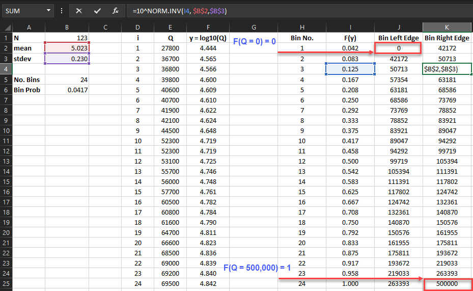
The cumulative frequency at each bin is computed as the bin number, $\begin{array}{l}i\end{array}$ , multiplied by the bin probability of 0.0417.

For each bin, the discharge denoting the right bin edge is the quantile corresponding to the CDF value for the bin. The quantile value is computed using the Excel function NORM.INV. The function arguments are the cumulative frequency, $\begin{array}{l}F(y_i)\end{array}$ , mean of the base 10 logarithm of discharge, and standard deviation of the base 10 logarithm of discharge. The function NORM.INV returns the quantile, which is the base 10 logarithm of the discharge. To calculate the discharge value corresponding to the right edge of the bin, raise the number 10 to the quantile value.

The discharge denoting the left bin edge is equal to the discharge denoting the previous right bin edge.

The left bin edge for the first bin was assigned a value of 0 cfs since the cumulative frequency to the left of the first bin equals 0. The right bin edge for the last bin was assigned a value of 500,000 which is greater than the largest observed discharge value. The cumulative frequency at the right edge of the last bin is equal to 1.

Compute the number of observed data values in each bin. This is the observed frequency, or $\begin{array}{l}O_i\end{array}$ . Use the Excel function COUNTIF.

To determine the number of observed discharges in each bin, calculate the difference between the number of values less than the right edge of the bin and the number of values less than the left edge of the bin.

Check that your formula is correct by summing the observed frequency column. The sum of the observed frequency column should equal $\begin{array}{l}N\end{array}$ , the number of data points.

Compute the expected frequency of each bin, or $\begin{array}{l}E_i\end{array}$ : $\begin{array}{l}E_i = \frac {N}{Number of Bins}\end{array}$
Calculate the Chi-Squared test statistic, $\begin{array}{l}\chi^2\end{array}$ .

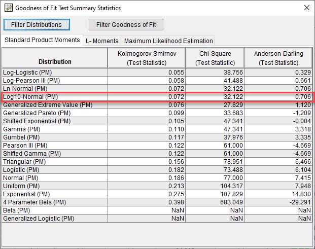
The computed Chi-Squared test statistic is 32.122. This matches the value from Distribution Fitting Test 20 in the HEC-SSP Examples.

Question: Based on the K-S and C-S test statistics computed for the 19 analytical distributions in HEC-SSP, is the log-normal distribution a good choice for the annual peak discharge data from the Point of Rocks gage?

Distributions with smaller values of the K-S and C-S test statistics are considered better at describing the data. Small K-S and C-S test statistics indicate small differences between the observed and expected frequencies. The Log10-Normal distribution produces relatively low test statistics compared to the other distributions in HEC-SSP. The Log-Logistic, Log Pearson III, Generalized Extreme Value, and Ln-Normal distributions produce K-S and C-S test statistics that are smaller than or equal to those from the Log10-Normal distribution. When selecting a distribution, it is important to not only consider the goodness of fit test statistics but the applicability of the distribution to the data.

If time allows, continue to Task 4. Anderson-Darling Test.