Download PDF
Download page Task 3. Fit and Compare Multiple Models to the Winter Season 3-day Precipitation Time Series.
Task 3. Fit and Compare Multiple Models to the Winter Season 3-day Precipitation Time Series
Now that you’ve performed an initial analysis of the SWE and precipitation data and determined that multiple flood seasons are of interest, you can begin to fit and evaluate different models. As was previously mentioned or deduced, multiple types of storms/floods affect the Willamette River watershed. When multiple storm or flood types are combined within an annual maximum series, the assumption of having an identical distribution can become tenuous, which affects the ability to make inferences about rare storms/floods. Additionally, the behavior of the right-hand tail typically used in dam and levee safety studies may be dominated by a storm/flood type that is less dominant in the more-frequent part of the accepted all-season variable-frequency model. Treating multiple storm and/or flood types as separate, independent and identically distributed samples allows for examination of the frequency of storms and/or floods per type. A mixed population analysis can then be used to combine the models fit to each storm and/or flood type into a single probability distribution that reflects the occurrence of more than one type per year. A mixed population analysis will not be performed as part of this workshop due to time constraints. However, it will be investigated as part of later workshops within the Flood Frequency Analysis class.
The first parametric modeling analysis will be focused on the winter season 3-day precipitation time series. Before fitting any models, use the tools contained within the Distribution Fitting | Data tab to create a representative, independent, and identically distributed sample for this season.
- Create a new Distribution Fitting analysis and name it “Detroit_3day_Winter”.
- Select the DETROIT DAM 3DAY PRECIP data set within the Data Set drop down menu.
- On the Data tab, ensure that Precipitation is selected within the Parameter Type drop down and click on the Filter Data button.
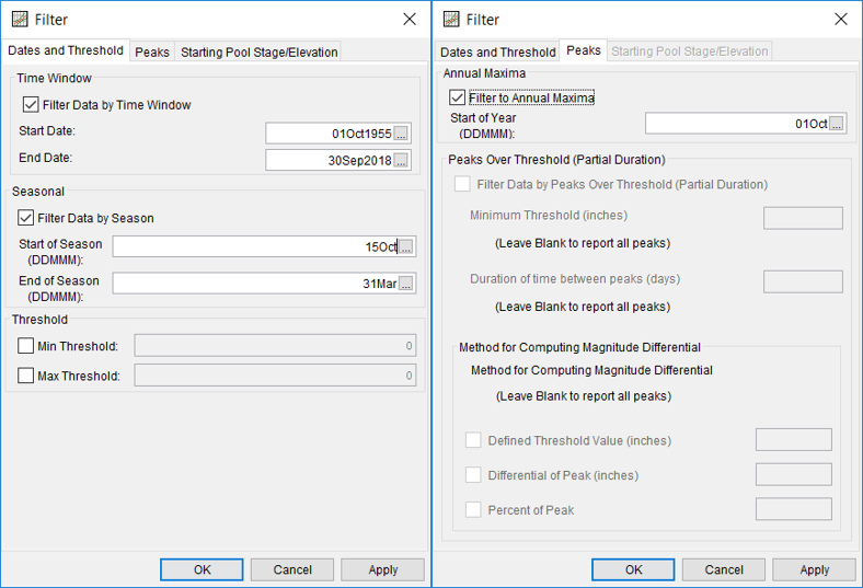
- Within the Filter editor, on the Dates and Threshold tab, click the Filter Data by Time Window box and enter a Start Date and End Date of 01Oct1955 and 30Sep2018, respectively.
- Also, click the Filter Data by Season box and enter a Start of Season and End of Season of 15Oct and 31Mar, respectively.
- Move to the Peaks tab and click the Filter to Annual Maxima check box. Enter a Start of Year of 01Oct.
- The Dates and Threshold tab and Peaks tab should appear similar to Figure 1.
- Click OK to apply the filters and close the editor.
- The Data tab should appear similar to Figure 2 (select the XY radio button for the time series plot).
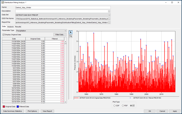
Question 8: How many values were contained within the original data set? After applying the filters, how many values remain?
Use the Data Summary Statistics.
23471 values were contained within the original data set. 63 values remain within the filtered/processed data.
Question 9: Can you find any water years in which 3-day precipitation accumulations within the winter season (i.e. 15Oct to 31Mar) in excess of four inches were filtered? How do you feel about not including that information within the analysis and potentially including smaller peaks in their place?
3-day precipitation accumulations within the winter season in excess of four inches are filtered multiple times including Feb 1961, Jan 1965, and Jan 2011. This information could be included if you were to construct a partial duration series instead of an annual maximum series.
Once you are satisfied with the data set, you can move on to the Analysis tab to begin fitting multiple models:
- Click the Apply button in the lower right corner of the Distribution Fitting editor, switch to the Analysis tab, and within the Distribution Filter panel, click the radio button to Display All Distributions.
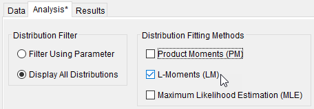
- Within the Distribution Fitting Methods panel, select the L-Moments (LM) checkbox, as shown in Figure 3. This will switch the fitting method from standard product moments to linear moments.
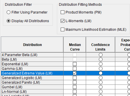
- Click on the left-most check box in the table to display the median curve for the Generalized Extreme Value | LM model choice, as shown in Figure 4.
- Try multiple distribution and fitting method choices. Be sure to use the Distribution Fitting analysis’ various plots, tabular data, and tools to visualize each model’s goodness of fit relative to the data. Also, try viewing the PDF, PP Plot, QQ Plot, and CDF-Plotting Position
Question 10: Which distributions provide arguably the best fit to the data when using the Linear Moments fitting method? Why do you think that is the case? Are there any distributions within that family that do not provide adequate fits? Why?
The Generalized Extreme Value (GEV), Generalized Logistic (GLO), and Gumbel distributions provide roughly equally good fits to the data when using the Linear Moments fitting method (based on the Kolmogorov-Smirnov test statistic). The GEV and GLO distributions, along with the Generalized Pareto (GPA) distribution belong to the family of three-parameter distributions with a common parameterization scheme devised by Hosking and Wallis (1996), each using a location ξ, scale α, and shape κ parameter. These distributions are commonly used within precipitation-frequency analyses, most notably the National Oceanic and Atmospheric Administration (NOAA) Atlas 14 volumes. In fact, the GEV distribution is directly derived by taking the maximum of repeated independent samples from a homogeneous population, which is what was used to derive the annual maximum series in this analysis.
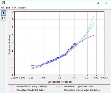
However, the GPA distribution does not provide as adequate a fit to the data as the GEV or GLO distributions nor is it appropriate to extrapolate and estimate quantiles for rare exceedance probabilities, as is required within this analysis. This is shown in Figure 5. This is due to the derivation of the GPA distribution. An underlying assumption of the GPA is that subsamples exceeding a sufficiently high threshold from repeated samples of a homogeneous population converge to the GPA distribution. In other words, if repeated samples are taken from a population, and only the values in those samples that are greater than a selected value are retained, then those retained values will follow the GPA distribution. However, this type of data set (partial duration series) is not what was used in the analysis. If one were to filter the input data set in a different way to extract a partial duration series, the GPA distribution may provide a better fit.
- Once you have determined an acceptable distribution and fitting method, click the corresponding radio button within the Accept Distribution column. This will compute the confidence limits and expected probability curve (if they weren’t already computed).
- Move to the Results tab. Within this tab, you will find statistics and parameters related to the original data, filtered data, selected distribution and fitting method, selected goodness of fit method, as well as the computed frequency curves.
Question 11: Which model did you choose? What were its parameters? What is the resulting 10-, 2-, 1-, 0.5-, and 0.2-percent chance exceedance 3-day precipitation accumulations for the winter season?
The GEV | Linear Moments model was chosen. However a case could also be made to choose the GLO | Linear Moments or Gumbel | Linear Moments models instead. The location, scale, and shape parameters for this model were 2.914, 0.706, and -0.016, respectively. The resultant 10-, 2-, 1-, 0.5-, and 0.2-percent chance exceedance 3-day precipitation accumulations for the winter season were 4.53, 5.06, 5.76, 6.28, 6.82, and 7.53 inches, respectively.
- Click the OK button to close the Distribution Fitting analysis editor.
- Click the Save button to save the study.
Continue to Task 4. Fit and Compare Multiple Models to the All-Season SWE Time Series.