Workshop Files

Download the workshop files here:

MixedPopulationsWorkshop.Rpds_events.RData

Software

The following software was used to create this example:

HEC-SSP v2.3-beta 5: https://www.hec.usace.army.mil/software/hec-ssp/download.aspx

CRAN R version 4.2.2 or newer

RStudio version 2023.03.0+386 or newer

Introduction

In fitting an analytical probability distribution to a sample of flood events, we make the assumption that the flood events are independent and identically distributed (IID). At many locations in the United States, floods are produced by multiple mechanisms. A flood series comprised of floods caused by different physical processes is called a mixed population. We are violating the "identically distributed" assumption at sites where floods are caused by multiple mechanisms. The "identification and treatment of mixed distributions" was listed in the Future Studies section of the latest two versions of Federal flood frequency guidelines, Bulletin 17B (1982) and Bulletin 17C (2019).

The method used in this tutorial to identify flood causal mechanism is one possible way to separate flood events in a mixed flood series. This tutorial is not Federal guidance.

Site Information: Merced River

The Merced River originates in the Sierra Nevada and flows through Yosemite National Park, before joining the San Joaquin River in the Central Valley of California. This tutorial will investigate floods at USGS 11266500 Merced River at Pohono Bridge near Yosemite, CA. The gage has a drainage area of 321 square miles. Annual peak flows at the gage are available starting in WY1918 and continuous mean daily streamflow data is available starting in WY1917.

Major Floods in Yosemite National Park

National Park Service video of May 1996 and January 1997 floods in Yosemite National Park

Heavy Precipitation Event Southwest Oregon, Northern California, and Western Nevada December 26, 1996 - January 3, 1997

This workshop has four tasks and will use HEC-SSP and R to compute the results.

1. Examine flood event data in HEC-SSP
2. Compute flood event contributions from rain and snowmelt
3. Investigate the sensitivity of flood type classification to thresholds
4. Fit analytical probability distributions to flood type subsets

Task 1: Examine Flood Event Data in HEC-SSP

1. Open HEC-SSP v2.3 beta.5.
2. Create a new study by selecting File | New Study... (or use the keyboard shortcut Ctrl+N).
3. Enter "MercedRiver" as the Study Name. Leave the Unit System set to English and the Coordinate System set to Geographic.
4. Save the file in an appropriate directory and click the OK button.
5. Open the Data Import Wizard by selecting Data | New | Using Import Wizard... or by right-clicking on the Data folder and selecting New | Using Import Wizard....
6. Leave the default selections on the Create New Data Set screen of the data importer. Click the Next> button.
7. Select the radio button next to USGS Website and click the Next> button.
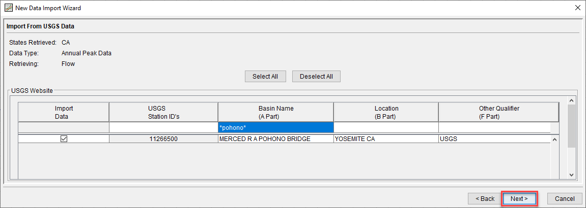
8. Leave the default selections for the Data Type and Retrieve Data for sections (Annual Peak Data and Flow, respectively).
9. In the Station ID's section, select Get USGS Station ID's by State. Click the Get ID's for State button and select California.
10. Click the OK button to close the dialog box. Click the Next> button.
11. In the Basin Name (A Part) column, enter *pohono*.
    
    

    The asterisk (*) can be used as a wildcard to search for all strings that contain what has been typed.

12. Check the box next to USGS 11266500 Merced River at Pohono Bridge, CA.
13. Click the Next> button. 
    
14. Click Import.
15. When the import is complete, open the data importer again. 
16. Leave the default selections on the Create New Data Set screen of the data importer. Click the Next> button.
17. Select the radio button next to USGS Website and click the Next> button.
18. Change the Data Type to Daily. Under Daily Options, check the box next to Retrieve Period of Record and select UTC as the time zone.
19. Select California in the Station ID's section.
20. Search for the gage and check the box next to USGS 11266500 Merced River at Pohono Bridge, CA.
21. Click Next> and Import.
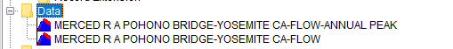
22. You should have two datasets in the Data folder.
    
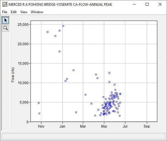
23. Right click on the Annual Peak dataset and select Year-Over-Year Plot. 
    
24. Leave the Year Specification as Water Year (starts Oct 1). Click Plot.

    QUESTION 1. What do you notice about the seasonality/timing of annual peak flows?

    ANSWER 1

    The timing of annual peak flows exhibits strong seasonality. Most annual peak flows occur in the spring (April - June) and coincide with spring snowmelt. However, the springtime annual peak floods tend to have smaller magnitudes than events that occur in the fall and winter months. The fall and winter flood events at this site are up to 10x larger than springtime floods. 

    

    
    

25. Create a new Bulletin 17 analysis by right-clicking on the Bulletin 17 folder and selecting New....
26. Enter "MercedRiver_B17C" as the Name.
27. Select the Annual Peak dataset from the Flow Data Set drop-down menu.
28. Leave the default selections on all tabs. Click Compute.

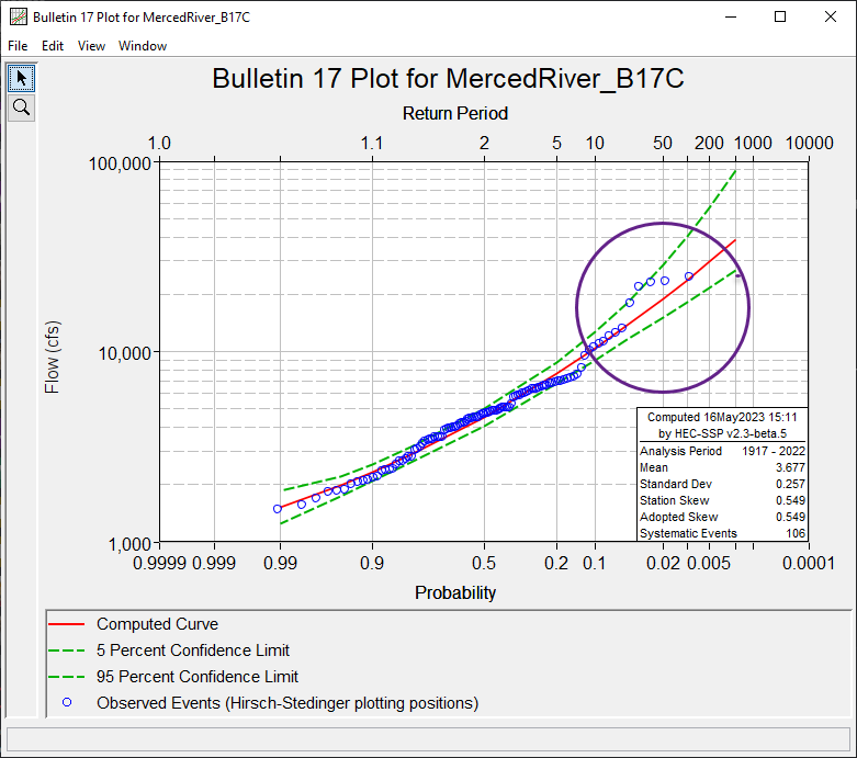
29. Click Plot Curve.
    
    QUESTION 2. What do you notice about the fit of the LP3 curve?

    ANSWER 2

    The plotting positions have a pronounced S-shape which is indicative of multiple flood causal mechanisms. The fit of the LP3 distribution to the data isn't great at the upper end of the curve.

    

    
    

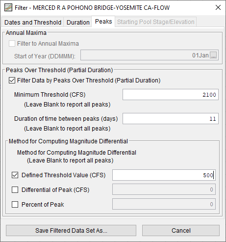
30. Next, extract a Partial Duration Series (PDS) from the mean daily streamflow data. Right-click on the daily streamflow dataset and select Filter Data...
    
31. Select the Peaks tab.
32. In the Peaks Over Threshold (Partial Duration) section, check the box next to Filter Data by Peaks Over Threshold (Partial Duration).
33. The flood separation and threshold values were determined using the procedures described in Flood Separation and Threshold Choice Workshop. Diagnostic plots (the threshold-event trade-off plot, the Pareto shape parameter plot, and the mean excess plot) were used to determine an appropriate flow threshold. A time-based separation with recession was used. A minimum separation of 11 days (computed using the $//<![CDATA[ \begin{array}{l}\lceil 5+\ln(DA) \rceil\end{array} //]]>$ rule) and recession threshold of 500 cfs were used.
    
    

    Where does 5 + ln(DA) come from?

    The $//<![CDATA[ \begin{array}{l}\lceil 5+\ln(DA) \rceil\end{array} //]]>$ computation is included in Appendix 14 of Bulletin 17 (1976) and Bulletin 17B (1982) to ensure independence between events. 

34. Enter the following:
    1. Minimum Threshold (CFS): 2100
    2. Duration of time between peaks (days): 11
35. In the Method for Computing Magnitude Differential section, check the box next to Defined Threshold Value (CFS). Enter a value of 500. 
    
36. Click Save Filtered Data Set As....
37. Name the new dataset as in the image below.
    
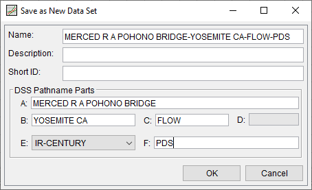
38. Click the OK button.
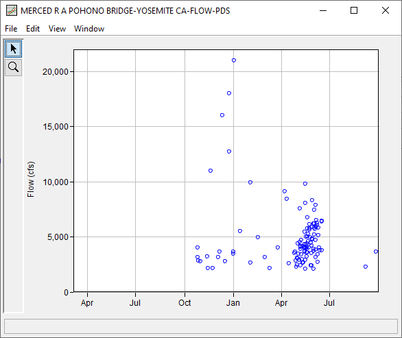
39. Right click on the newly created PDS dataset and select Year-Over-Year Plot.
    

    QUESTION 3. What do you notice about the seasonality/timing of PDS flood events?

    ANSWER 3

    The timing and seasonality of the PDS flood events is the same as that of the annual peak flows (see ANSWER 1).

    

Task 2: Compute PDS Flood Event Contributions from Rain and Snow

1. Download the MixedPopulationsWorkshop.R script and the pds_events.Rdata file to the same folder on your computer.
2. In RStudio, set the working directory to the file directory containing these files. 
3. Open the MixedPopulationsWorkshop.R script in RStudio.
4. Run lines 1-54. This will load libraries, load mean daily streamflow data for WY1982-2021 using the dataRetrieval library, extract the annual maximum daily flow, load the previously developed partial duration series data frame, and plot the mean daily flow (PDS as blue diamonds and AMS as magenta circles). Note that the AMS and PDS were developed from the mean daily flow time series.
   
   QUESTION 4. How many events are in the AMS and PDS? Are there differences between the PDS and AMS?
   
   ANSWER 4

   The AMS is comprised of 41 events since we are working with 41 years of streamflow record. The PDS is comprised of 44 events.

   Most of the events in the AMS were also selected in the PDS. However, the PDS includes multiple events per year in WY 1982, 1983, 1997, and 2017 and does not include smaller annual peak flows in WY 1988, 2014, 2015, and 2021.

   

   
   Steps 2-5 were performed for you. In Task 3, you will classify the partial duration series events during the period WY 1982-2021 by flood causal mechanism. The time period WY 1982-2021 corresponds to the availability of spatially distributed snow-related data from the University of Arizona dataset.
5. Define an antecedent period to compute relevant meteorologic indices for flood type attribution. In this tutorial, an antecedent period of $//<![CDATA[ \begin{array}{l}\lceil 5+\ln(DA) \rceil\end{array} //]]>$ where DA is in square miles, was used. 
6. Compute basin-average cumulative precipitation during the event antecedent period using the Livneh et al. (2013) precipitation dataset for WY1982-2011 events.
7. Compute basin-average cumulative precipitation during the event antecedent period using the National Weather Service Analysis of Record for Calibration (AORC) dataset for WY2011-2021 events.
8. Compute basin-average maximum decrease in snow water equivalent (SWE) during the event antecedent period using the University of Arizona (UA) dataset.

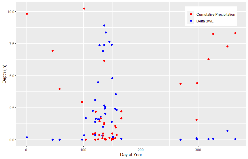
Run lines 57-65 to plot the depths of precipitation and snowmelt contributing to each PDS event against day of year.

QUESTION 5. What do you notice about the relative contribution from precipitation vs. snowmelt before flood events in the PDS?

Task 3: Investigate Sensitivity of Flood Type Classification to Thresholds

Step 1: Use Absolute Thresholds to Separate Rain and Snowmelt Events

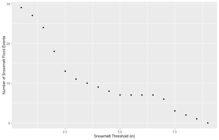
Run lines 70-82 to plot the number of floods classified as snowmelt events against the snowmelt threshold in inches.

QUESTION 6. How many events were classified as snowmelt- and rain-driven using various snowmelt contribution (in) thresholds?

Step 2: Use Relative Thresholds to Separate Rain and Snowmelt Events

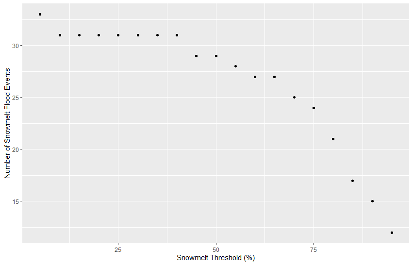
Run lines 85-97 to plot the number of floods classified as snowmelt events against the snowmelt threshold in %.

QUESTION 7. How many events were classified as snowmelt- and rain-driven using various snowmelt contribution (%) thresholds?

Task 4: Fit Analytical Probability Distributions to Flood Type Subsets

In this task, you will compute mixed (i.e. no separation) and combined frequency curves. The combined frequency curve will be developed using the probability of union. The combined exceedance probability is computed as:

$//<![CDATA[ \begin{array}{l}P_c = 1 - \prod_{i=1}^{n} (1 - P_i)\end{array} //]]>$ which simplifies to $//<![CDATA[ \begin{array}{l}P_c = 1 - (1 - P_r_a_i_n)(1 - P_s_n_o_w) = P_r_a_i_n + P_s_n_o_w - P_r_a_i_n * P_s_n_o_w\end{array} //]]>$ for two populations.

The combined non-exceedance probability is computed as:
$//<![CDATA[ \begin{array}{l}F(x) = 1 - P_c = F_r_a_i_n(x)*F_s_n_o_w(x)\end{array} //]]>$

Step 1: Use a 75% Snowmelt Contribution Threshold

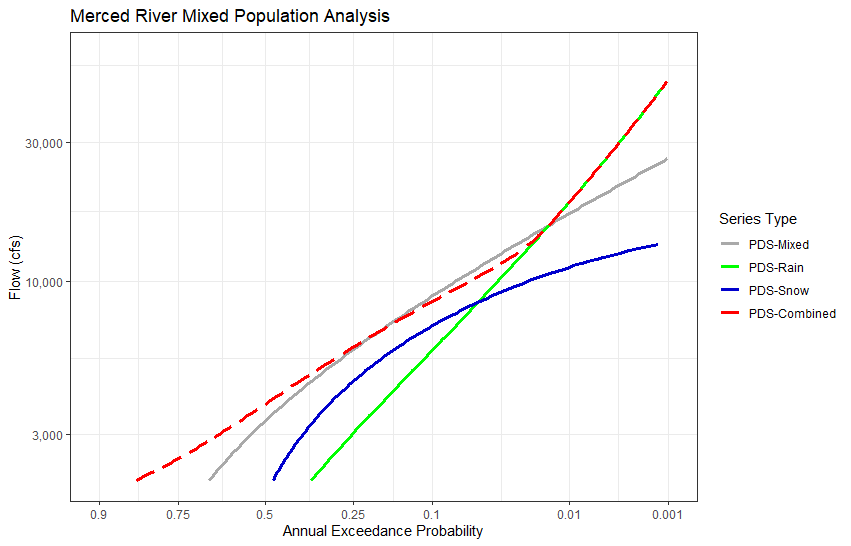
Run lines 101-155. This will (1) divide the PDS into rain and snowmelt events using a 75% snowmelt contribution threshold, (2) fit the generalized Pareto distribution to the mixed (i.e. no separation), rain, and snowmelt floods using L-moments, (3) generate flows ranging from the threshold value to 60,000 cfs, (4) compute the annual non-exceedance probability for each of the generated flows using the Langbein adjustment, (5) compute the combined frequency curve using probability of union, (6) plot the frequency curves, and (7) compute the 1% and 0.1% annual exceedance probability (AEP) quantiles from the mixed and combined curves.

Note that probabilities computed from the functions lmomco::cdfgpa and lmomco::fpds2f are non-exceedance probabilities. The frequency curve x-axis labels were replaced with AEP as is common in hydrology.

QUESTION 8. What is the generalized Pareto distribution shape parameter for the mixed (i.e. no separation) flood series? View the gp_mixed variable in the Environment tab.

QUESTION 9. Using a 75% snowmelt contribution threshold, how many PDS flood events were classified as snowmelt- and rain-driven? What is the generalized Pareto shape parameter for each flood subset? What is the difference in the 1% and 0.1% AEP quantiles between the mixed and combined curves (view the qua_combined, qua_mixed, and qua_diff variables in the Environment tab)?

Step 2: Use a 1.25 in Snowmelt Contribution Threshold

Run lines 158-206. This will perform the same computations described in Step 1 but the PDS will be divided into rain and snowmelt events using a 1.25 inch snowmelt contribution threshold.

QUESTION 10. Using a 1.25 in snowmelt contribution threshold, how many PDS flood events were classified as snowmelt- and rainfall-driven? What is the generalized Pareto shape parameter for each flood subset? What is the difference in the 0.1% AEP flow quantile between the mixed and combined curves (view the qua_combined, qua_mixed, and qua_diff variables in the Environment tab)?

QUESTION 11. Comment on the differences between the parameters obtained using a 75% and 1.25 in snowmelt contribution threshold. Also, comment on the differences in the generalized Pareto distribution parameters between the mixed, rain, and snow populations. 

QUESTION 12. Do you think that 2 populations (rain and snowmelt floods) are sufficient to describe floods at this site? If not, why?