Download PDF
Download page Task 2. Investigate Threshold Sensitivity.
Task 2. Investigate Threshold Sensitivity
Background
The most challenging part of a peaks over threshold analysis is selecting an appropriate threshold value. A high threshold helps ensure the sample consists of true flood events. However, setting the threshold too high can produce an small sample size and may violate the assumption that the fitted model is representative of the underlying population. Conversely, setting the threshold too low can include non-extreme events into the sample.
In addition to using a representative sample, the sample values should be independent of each other. To ensure independence, time separation and magnitude differential criteria can be applied. Time separation criteria ensure that enough time has passed between events. Magnitude differential criteria ensures that the hydrograph has sufficiently receded between floods. Magnitude differential criteria are less applicable to other variables that do not exhibit serial correlation, such as precipitation.
Task Outline
In this task, we will first extract partial duration series using a single time separation criterion while varying the threshold value. We will compare the following properties of each partial duration series:
- Number of events
- Mean rate of events
- Mean excess (which expresses the average amount your PDS exceeds the threshold by)
- Generalized Pareto Distribution parameters
- Anderson-Darling right tail weighted test statistic
Threshold from Diagnostic Plots
- Select the Filtering tab.
- In the Threshold Selection panel, leave the Selected Threshold field blank. Check the box next to Investigate Partial Duration Threshold Value.
- Enter the following:
- Minimum Threshold (CFS): 500
- Maximum Threshold (CFS): 7000
- Number of Thresholds: 100
Threshold Selection
The user can elect to compute diagnostic quantities for 10 to 100 threshold values (Number of Thresholds). If the user enters a Number of Thresholds value less than 10 or greater than 100, the HEC-SSP will display a warning message. The Minimum Threshold and Maximum Threshold values should be set such that 10 to 100 thresholds and the corresponding diagnostic data provides enough information for selection of a single threshold. The range specified by the Minimum Threshold and Maximum Threshold can be set wide initially, then narrowed iteratively.
The diagnostic plot quantities (discussed later) will then be computed for each threshold value.
- In the Time Separation Between Peaks panel, check the box next to Apply Time Separation Criterion.
- Select the second radio button, next to ceiling[5 + ln(Drainage Area)]. Enter the gage's drainage area, 106 (square miles), in the field.
Time Separation Between Peaks
Multiple time separation criterion can be utilized to further refine the filtered time series. "Time separation" refers to an amount of time that must elapse before another peak is identified. Two time separation method choices are available for user: User-specified and ceil[5 + ln(DA)].
- The User-specified option allows the user to enter a time duration, in days, between peaks.
- The second option uses an equation, provided in Bulletin 17, that is used as a time separation criterion to ensure independence between partial duration series flood events (U.S. Water Resources Council, 1976). The equation is:
t = ceil[5 + ln(DA)]
where t is the time duration (days), ceil is the ceiling function (returns the smallest integer greater than or equal to the argument), and DA is the drainage area (square miles).- This equation is relevant when applying a Peaks Over Threshold Analysis to streamflow events.
- A streamflow gage with a drainage area of 106 square miles, such as the one used in this workshop, has a time separation of ceil[5 + ln(106)] = ceil(9.7) = 10 days.
- Do not select or enter anything in the Method for Computing Magnitude Differential panel.
For more information pertaining to the multiple Magnitude Differential options, navigate to the Filtering Data | Peaks Tab section of the User's Manual.
- The Filtering tab should appear as in the image below:

- Click the Plot Threshold Selection Diagnostic Plots button. The Threshold Selection Diagnostic Plots dialog, with 5 plot panels, will appear.

- To see these values in tabular format, select File | Tabulate from the top ribbon of the plot dialog.
Diagnostic Plots
Five diagnostic plots are produced: number of exceedances, rate of exceedances, Generalized Pareto distribution shape parameter, mean excess, and the Anderson-Darling right tail weighted test statistic. Each of these quantities is plotted against threshold value.
Number of Exceedances
The number of exceedances is the sample size of the partial duration series. For example, 50 exceedances of the threshold means that there are 50 events in the PDS.
Rate of Exceedances
Using an average rate of 1 event per year as a criterion ensures that the partial duration series and annual maximum series have the same sample size. There is no special meaning beyond that but this criterion can be useful in the absence of other information.
Generalized Pareto Distribution Shape Parameter
The smallest threshold value corresponding to a stable shape parameter is selected (Naghettini, 2017). The Generalized Pareto distribution shape parameter is fitted using the Distribution Fitting Method selected on the General tab.
Mean Excess
Typically, the threshold value is selected when the mean residual life plot’s behavior becomes nonlinear, or there is a break in the slope (Naghettini, 2017).
Anderson-Darling Right Tail Weighted Test Statistic
Solari et al. (2017) proposed a method for automated threshold selection, based on an empirical distribution function (EDF)-statistic and a goodness-of-fit test to test the null hypothesis that exceedances of a high threshold come from a Generalized Pareto distribution. The Anderson Darling A2 statistic is an EDF-statistic, which assigns more weight to the tails of the data than similar measures. Sinclair et al. (1990) proposed the right-tail weighted Anderson Darling statistic AR2 which allocates more weight to the upper tail and less to the lower tail of the distribution than A2 and is given by:
A_R^2=\frac{n}{2}-\[ \sum_{i=1}^{n} [(2 - \frac{2i - 1}{n}) ln(1 - z_i) + 2z_i] \]
where z = F(x) and n is the sample size.
You should see the following in the following message in the Message Window:
Warning: less than 25 values in the PDS
HEC-SSP provides a warning when a threshold value is high enough that there are less than 25 events in the resulting partial duration series. At this site, threshold values greater than 5,425 cfs resulted in partial duration series sample sizes less than 25.
- After investigating the threshold selection diagnostic plots, adjust the Minimum Threshold, Maximum Threshold, and/or the Number of Threshold values to produce a narrower range of threshold values. Re-plot the diagnostic plots.
- Choose a plausible threshold value from the lower end of the range used to generate the diagnostic plots.
- Enter the threshold in the Selected Threshold field.
Click the Refresh Plot button on the bottom of the General tab to visualize your threshold and the resulting partial duration series in the time series plot.
- Leave the Minimum Threshold, Maximum Threshold, and the Number of Threshold values unchanged.
Note the the Minimum Threshold, Maximum Threshold, and Number of Threshold values are not used in the analysis compute. These values are only used to generate diagnostic data values for investigation purposes.
- Leave the Time Separation criterion that you entered in the previous step.
- Click the Compute button.
- Investigate the results:
- Examine the selected partial duration series on the plot panel of the Filtering tab.
- Navigate to the Tabular Results tab.
- Click the Plot Curve button.
- Click the Plot Event Count Histogram button.
QUESTION 2: Report the threshold diagnostic data and flow quantiles (computed curve) for the selected threshold. What is the most frequent event count (events/year) in this partial duration series (hint: look at the Event Count Histogram)?
A "low" threshold value of 1,000 cfs was selected. This is the lower end of where both the shape plot and mean excess plot indicate stable behavior. The right-tail AD statistic also has a minimum value in this range. Your results will be different if you selected a threshold value other than 1,000 cfs.
The most frequent event count was 1 event per year:

| Diagnostic Data Statistic | Value |
|---|---|
| Number of Exceedances | 175 |
| Rate of Exceedances | 1.99 |
| Generalized Pareto Shape Parameter | -0.083 |
| Mean Excess (cfs) | 2,273 |
| Anderson Darling Right Tail Weighted Test Statistic | 0.186 |
The flow frequency quantiles presented below are for the annualized frequency curve, meaning that the quantiles correspond to annual exceedance probabilities (AEPs). Probabilities obtained from the Generalized Pareto distribution are conditional probabilities - they describe the probability of exceeding some value x, given that they have already exceeded the threshold value, u: P(X > x | X > u). An extra step, called annualization, is needed to convert the conditional probabilities to AEPs. HEC-SSP performs annualization for the user!
| AEP | Computed Curve Flow (cfs) |
|---|---|
| 0.2 | 19,900 |
| 0.5 | 16,730 |
| 1.0 | 14,490 |
| 2.0 | 12,360 |
| 5.0 | 9,710 |
| 10.0 | 7,790 |
| 20.0 | 5,920 |
| 50.0 | 3,300 |

- Click OK to close the "SanLorenzo_Low" analysis.
- Save the SSP study.
- Right click on the "SanLorenzo_Low" analysis and select Save As....
- Enter "SanLorenzo_High" as the analysis name and change the description to "Investigation of high threshold".
- Click OK to create the new analysis.
- Open the new analysis and select the Filtering tab.
- Choose a plausible threshold value from upper end of the range used to generate the diagnostic plots. Enter the threshold in the Selected Threshold field.
- Leave the Time Separation criterion that you entered in the previous step.

Click the Refresh Plot button to update the plot panel and to see how the partial duration series changes based on the filtering criteria. The plot will automatically refresh when the analysis is computed.

- Click the Compute button.
- Investigate the results:
- Navigate to the Tabular Results tab.
- Click the Plot Curve button.
- Click the Plot Event Count Histogram button.
QUESTION 3: Report the threshold diagnostic data and flow quantiles (computed curve) for the selected threshold. What is the most frequent event count (events/year) in this partial duration series (hint: look at the Event Count Histogram)?
A "high" threshold of 3,000 cfs was selected. Your results will be different if you selected a threshold value other than 3,000 cfs.
The most frequent event count was 0 events per year:
Using a threshold of 3,000 cfs reduced the number of events in the PDS from 175 to 67 and the average rate of exceedances from almost 2 events per year to 0.77 event per year. However, increasing the threshold from 1,000 cfs to 3,000 cfs had very little impact on the Generalized Pareto shape parameter (-0.083 vs. -0.082)
| Diagnostic Data Statistic | Value |
|---|---|
| Number of Exceedances | 67 |
| Rate of Exceedances | 0.761 |
| Generalized Pareto Shape Parameter | -0.082 |
| Mean Excess (cfs) | 2,423 |
| Anderson Darling Right Tail Weighted Test Statistic | 0.229 |
The high threshold estimate results in a mean rate less than 1 event per year, which isn't a deal breaker but is worth re-considering, especially if a review of the historical time series shows that flows less than this threshold are still important to capture and can happen multiple times per year, and this is more likely to happen than no significant floods in a year.
| AEP | Computed Flow (cfs) |
|---|---|
| 0.2 | 20,430 |
| 0.5 | 17,140 |
| 1.0 | 14,800 |
| 2.0 | 12,590 |
| 5.0 | 9,830 |
| 10.0 | 7,840 |
| 20.0 | 5,880 |
| 50.0 | 3,150 |

- Click OK to close the "SanLorenzo_High" analysis.
- Save the SSP study.
Threshold at Bankfull Discharge
Another method to select a flow threshold is bankfull discharge. At many sites, bankfull discharge can be a useful starting estimate for a threshold that divides routine (in-channel) flows from flood flows. There are several ways to estimate the bankfull discharge. One way is to use regional regression equations to estimate bankfull channel geometry, and then use Manning's equation with some assumptions to back into a bankfull discharge. These values can be obtained from USGS StreamStats. Another way is to use flow measurements at the site and look for an inflection point in the rating curve, such as in the plot below:
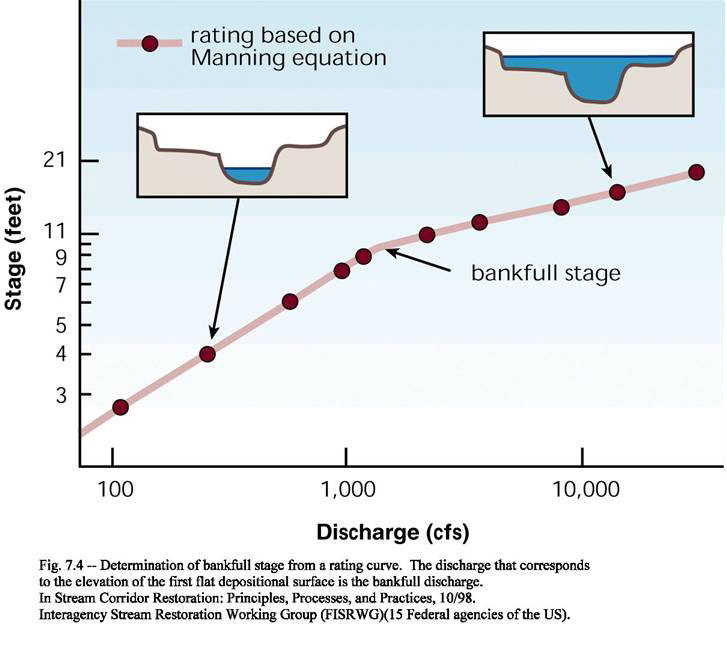
Measurements at the site go back to 1937 but the channel has changed significantly over time. Using R, a rating curve was developed using the last 10 years of data (WY2013-22):
")
QUESTION 4: Can you estimate bankfull discharge for this gage from this plot? If so, what is its value? If not, why not?
For this site, the channel is deeply incised and the rating curve shows no signs of inflection - it is concave up across the entire range of discharges. There is no clear point where we could pick up an estimate for bankfull discharge based on the measurements.
In fact, there is a journal paper about this very site reaching the same conclusion: https://onlinelibrary.wiley.com/doi/10.1002/esp.5299 It remarks that only a couple of events have exceeded the bankfull stage in the record. Bankfull discharge will not be a useful tool to find a threshold here.
As an extra note, if you use the regional geomorphologic regression equations from StreamStats, it results in nonsensical geometry when solving for an equivalent trapezoidal shape.
In the event that you want to test an estimated value for bankfull discharge, create a new Peaks Over Threshold analysis named "SanLorenzo_Bankfull" and enter your threshold on the Filtering tab in the Selected Threshold field. Leave the other filtering criteria unchanged.
Threshold at Minimum Annual Maximum
Using the minimum annual maximum flow has two advantages: (1) it is easy to compute and (2) it ensures all your AMS events are also in your PDS. However, it has some drawbacks. For ephemeral streams, or streams that have years during which no flows would be classified as floods, this approach can yield a threshold that is too low and results in selecting too many peaks.
- Right click on the "SanLorenzo_High" analysis and select Save As....
- Enter "SanLorenzo_MinAnnualMax" as the analysis name.
- Open the new analysis and select the Filtering tab.
- Enter the minimum annual maximum value, 128 (cfs), in the Selected Threshold field.
- Click the Compute button.
- Investigate the results:
- Navigate to the Tabular Results tab.
- Click the Plot Curve button.
- Click the Plot Event Count Histogram button.
QUESTION 5: What is the primary issue with using the minimum annual maximum threshold for this specific site?
The threshold corresponding to the minimum annual maximum is 128 cfs. This is a very low threshold and the low value indicates that this stream can experience prolonged periods of low flows and produce years where the largest flows are not floods. This value is well outside the range of the diagnostic plots and is likely to produce poor results.
Selection of an appropriate threshold is critical for peaks over threshold modeling because the exceedances above the threshold converge to the Generalized Pareto distribution if the threshold is sufficiently high (Extreme Value Theorem II). If the threshold is too low, convergence does not occur. In addition, using a threshold that is too low can violate the assumption that events are independent. Notice that multiple peaks from a single hydrograph/hydrologic event are retained in the PDS when a threshold of 128 cfs and 10-day time separation are used:
")
The event count histogram shows that the partial duration series contains a year with 12 events. This is a very high event count and indicates that the filtering criteria were not sufficient to ensure independence (i.e. the threshold is too low).

| Diagnostic Data Statistic | Value |
|---|---|
| Number of Exceedances | 536 |
| Rate of Exceedances | 6.091 |
| Generalized Pareto Shape Parameter | -0.385 |
| Mean Excess (cfs) | 1,211 |
| Anderson Darling Right Tail Weighted Test Statistic | 2.316 |
| AEP | Computed Flow (cfs) |
|---|---|
| 0.2 | 44,130 |
| 0.5 | 30,370 |
| 1.0 | 22,740 |
| 2.0 | 16,900 |
| 5.0 | 11,170 |
| 10.0 | 7,960 |
| 20.0 | 5,440 |
| 50.0 | 2,780 |

- Click OK to close the "SanLorenzo_MinAnnualMax" analysis.
- Save the SSP study.
Threshold at 1 Event Per Year
Using 1 event per year as a criterion ensures that the sample size is the same between the PDS and the AMS. It doesn't have any special meaning beyond that, but is a useful guideline absent any other information. You can determine the threshold that produces an average rate of 1 event per year by using the Threshold Selection Diagnostic Plots and selecting File | Tabulate from the top ribbon of the plot dialog. 
- Right click on the "SanLorenzo_MinAnnualMax" analysis and select Save As....
- Enter "SanLorenzo_1EventPerYear" as the analysis name.
- Open the new analysis and select the Filtering tab.
- Enter the threshold value corresponding to an average rate of 1 event per year in the Selected Threshold field.
The threshold corresponding to 1 event per year is about 2,650 cfs.
- Click the Compute button.
- Investigate the results:
- Navigate to the Tabular Results tab.
- Click the Plot Curve button.
- Click the Plot Event Count Histogram button.
QUESTION 6: How do you feel about the performance of the 1 event per year threshold at this site?
For this site, the 1 event per year criterion is not a bad choice when also considering the diagnostic plots. These results are not significantly different than the "high threshold" estimate, even with 20 additional events in the sample. This is a good sign that the results are relatively insensitive to threshold choice in this range. This is a very good fit to the data and produces quite reasonable results. This won't always work everywhere, especially in places where the variation in count per year in the PDS is significant, but is always worth a check.


| Diagnostic Data Statistic | Value |
|---|---|
| Number of Exceedances | 88 |
| Rate of Exceedances | 1.00 |
| Generalized Pareto Shape Parameter | -0.156 |
| Mean Excess (cfs) | 2,160 |
| Anderson Darling Right Tail Weighted Test Statistic | 0.249 |
| AEP | Computed Flow (cfs) |
|---|---|
| 0.2 | 22,550 |
| 0.5 | 18,250 |
| 1.0 | 15,380 |
| 2.0 | 12,790 |
| 5.0 | 9,750 |
| 10.0 | 7,690 |
| 20.0 | 5,770 |
| 50.0 | 3,270 |

- Click OK to close the "SanLorenzo_1EventPerYear" analysis.
- Save the SSP study.
Continue to Task 3. Investigate Separation Criteria.