Download PDF
Download page Task 2. Investigate the impact of regional skew for sites of different record lengths.
Task 2. Investigate the impact of regional skew for sites of different record lengths
Overview
This tutorial explores an example application of weighted skew using regional skew for two sites of varying record length. Bulletin 17C analyses will be created for each site using both station skew and weighted skew, and the resulting flood frequency curves for each site will be compared.
HEC-SSP version 2.3 was used to create this example. You will need HEC-SSP version 2.3, or newer, to open the project files.
Download a copy of the initial HEC-SSP project here (or continue using the project from Task 1): RegionalSkew_Start.zip
Introduction
This task will be performed using two analysis sites. These sites represent two hypothetical stream gages in central California: Foster Creek and Dixie Creek. The first gage, Foster Creek, represents a long gage record of 107 years (1905–2011). The second gage, Dixie Creek, represents a short gage record of 35 years (1945–1979). The watersheds are assumed to be of a similar drainage area and elevation. These data are used solely for the purposes of instruction and do not represent real data.
Open the HEC-SSP project and view the data. The figure below shows the Foster Creek and Dixie Creek annual maximum series plotted together.

Create a B17C Analysis using Station Skew
First, a Bulletin 17C analysis will be created for the longer gage, Foster Creek, using station skew.
- Create a new Bulletin 17 analysis called "Foster_Station Skew". Select the Foster Creek dataset from the dropdown. Ensure the 17C EMA and Use Station Skew methods are selected. Do not make any other changes to the General tab.
- It is always good practice to check for missing data. Select the EMA Data tab and examine the Flow Ranges table. There is no missing data so the analysis can continue.
- Select Compute to run the B17C analysis.
- View results using Plot Curve and in the Tabular Results tab. Make note of the Station Skew, Systematic Events, and Equivalent Record Length (years).
This process will now be repeated to create a Bulletin 17C analysis for the shorter gage, Dixie Creek.
- Create a new Bulletin 17 analysis called "Dixie_Station Skew". Select the Dixie Creek dataset from the dropdown. Ensure the 17C EMA method is selected. Do not make any other changes to the General tab.
- Select the EMA Data tab to confirm there is no missing data.
- Select Compute to run the B17C analysis.
- View results using Plot Curve and in the Tabular Results tab. Make note of the Station Skew, Systematic Events, and Equivalent Record Length (years).
The Foster Creek (long record) ERL is 107 years and the station skew is -0.144.
The Dixie Creek (short record) ERL is 34 years and the station skew is -0.144.
In this example, both sites have the same station skew — a fortunate coincidence that will help demonstrate the effects of using regional skew. In real applications, nearby sites having the same skew is extremely rare. Differences in physical features (like watershed slope or size), antecedent conditions (like soil moisture), and storm occurrence (like spatial orientation and timing) all contribute to the estimated distribution parameters of the sample population.


Look Up Regional Skew
Foster Creek and Dixie Creek are both located in the Central Valley of California. A regional skew study was completed by the USGS in 2011 (https://doi.org/10.3133/sir20105260). This study identified elevation as a meaningful predictor of regional skew. A linear regression model using mean basin elevation ("NL-Elev") provided the best estimate of regional skew over the other models that were considered. The NL-Elev model equation in Table 7 is summarized in Table 8 of the report.
Both Foster Creek and Dixie Creek have a mean basin elevation of approximately 2,000 ft. Based on the USGS regional skew study, this corresponds to an average regional skew of -0.50. The variance of prediction, VPnew, describes the estimated precision of the generalized skew and corresponds to the mean square error (MSE) used in Bulletin 17C. From the table, the MSE for both Foster Creek and Dixie Creek is 0.14.

Create a B17C Analysis using Weighted Skew
A Bulletin 17C analysis will be created for the longer gage, Foster Creek, using weighted skew.
- Create a new Bulletin 17 analysis called "Foster_Weighted Skew". Select the Foster Creek dataset from the dropdown.
- On the General tab, select Use Weighted Skew from the Generalized Skew options. Input -0.50 as the regional skew and 0.14 as the MSE.
- Select Compute to run the B17C analysis.
- View results using Plot Curve and in the Tabular Results tab. Make note of the Weighted Skew, Systematic Events, and Equivalent Record Length (years).
Repeat the process for Dixie Creek. Name the analysis "Dixie_Weighted Skew".
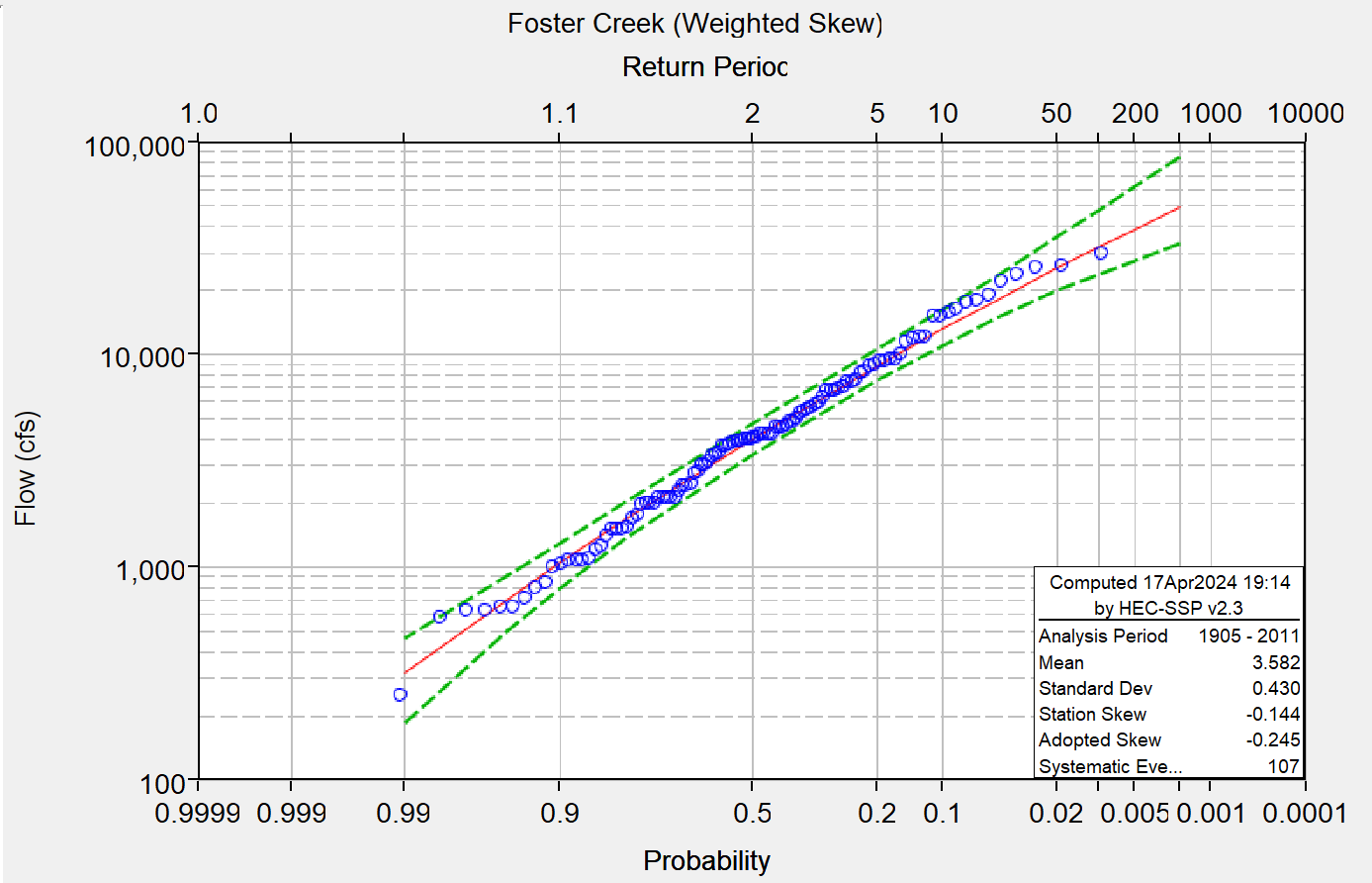
The Foster Creek (long record) ERL is 117 years and the weighted skew is -0.245.
The Dixie Creek (short record) ERL is 42 years and the weighted skew is -0.349.
As these sites are both located in central California and have a similar mean basin elevation, they both have a regional skew estimate of -0.50.

Comparison
For the long gage record, Foster Creek, the regional skew added an information content to the ERL of approximately 10 years (107 to 117). For the short gage record, Dixie Creek, the regional skew added an information content to the ERL of approximately 8 years (34 to 42).
The regional skew was more influential on the adopted skew for the short record than for the long record. For the long record, the adopted skew shifted from -0.144 (station) to -0.245 (weighted). For the short record, the adopted skew shifted from -0.144 (station) to -0.349 (weighted), which is closer to the regional skew estimate of -0.50. This is due to the weighting procedure for incorporating regional skew, as outlined in Bulletin 17C. The long record has a larger "weight" due to the larger sample size. The relative weight of the at-site skews can be compared by looking at the EMA Estimate of MSE (G at-site) output in the Tabular Results. For Foster, this value is 0.057 and for Dixie 0.155, meaning in the weighted skew computation, the at-site skew for Foster has almost three times the weight of the Dixie at-site skew when combining with the regional skew estimate. The weighting formula appears in equation 7-20 of Bulletin 17C.
In real applications, the regional skew value is especially important to improve the accuracy of estimates for gages with a short period of record.
The figures below show the analyses plotted together for each gage, with station skew displayed in green and weighted skew displayed in purple. Notice the width of the confidence bounds decreases for weighted skew due to the inclusion of additional information.


Download the final project files here: RegionalSkew_Finish.zip