Download PDF
Download page Coincident Frequency Analysis.
Coincident Frequency Analysis
This chapter discusses in detail how to use the Coincident Frequency Analysis editor in HEC-SSP. A coincident frequency analysis can be performed on any data type; flow, stage, precipitation, wind, etc. The coincident frequency analysis requires both duration and frequency curves. These can be computed by existing analyses in the HEC-SSP study or they can be entered manually in the Coincident Frequency Analysis editor.
Examples of this type of analysis can be found here:
Example when A and B can be Assumed Independent
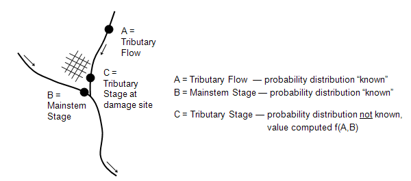
The Coincident Frequency Analysis is designed following guidelines in EM 1110-2-1415. This analysis tool can be used to compute the exceedance frequency relationship for a variable that is a function of two other variables. An example is illustrated in Figure 1. In this example, the stage at the damage site on the tributary, variable C, is a function of stream flow from the tributary, variable A, and the stage in the mainstem river, variable B.

The general procedure for performing a coincident frequency analysis, using HEC-SSP is described below.
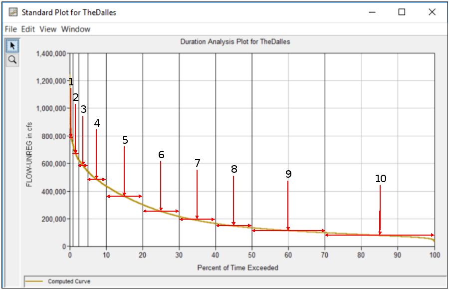
- Develop a duration curve for variable B. This can be done using the Duration Analysis editor or it can be defined manually in the Coincident Frequency Analysis editor. Then, discretize the duration curve to determine index values for variable B. The index values should be defined so that the area under the discretized duration curve approximates the original duration curve. Figure 2 shows a flow duration curve that has been discretized using 10 index points. The index points are taken at the midpoint of each discrete segment and there are more index points along the steeper portion of the duration curve. The Coincident Frequency Analysis editor can be used to define the index points and to estimate the proportion of time for each index point. For example, the 10th index point in Figure 2 is taken at the midpoint for the discrete segment from 100 to 70 percent of time exceeded. The flow value at this point represents the variable B index occurring 30 percent of the time. The 9th index point is taken at the midpoint for the discrete segment from 70 to 50 percent of time exceeded. The flow value at this point represents the variable B index occurring 20 percent of the time. The proportion of time assigned to each index point will be used to compute the variable C frequency curve.

- Different procedures are required depending on whether variables A and B are independent or not independent of one another. When variables A and B are assumed independent of one another, develop a frequency curve of variable A. The frequency curve can come from an existing Bulletin 17 or General Frequency Analysis or it can be defined manually in the Coincident Frequency Analysis editor. If variables A and B are not independent of one another, then develop a frequency curve of variable A for each variable B index value. In this case, the variable A frequency curves must be defined manually in the Coincident Frequency Analysis editor. This involves extracting annual peak values for variable A that occur for each discrete range identified on the variable B duration curve and performing a separate frequency analysis on each set of variable A data.
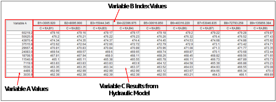
- Develop the response of variable C for combinations of variable A and variable B. This could be done using a hydrologic or hydraulic model. For the example shown in Figure 1, a flow value from the variable A frequency curve would be applied to the tributary and the index flow (or stage) from the variable B duration curve would be applied to the mainstem. The hydrologic or hydraulic model would be used to compute the variable C stage at some reference point on the tributary. This model simulation would be computed for many combinations of variable A and variable B. Figure 3 shows example output from a hydraulic model. The model was used to generate output from multiple combinations of variable A and B values. In this example, there were 12 variable A values and 9 index values from variable B. This resulted in 108 simulation results. The table shown in Figure 3 is referred to as the Response Curves table in HEC-SSP and these values must be entered by the user.

- The program computes the variable C frequency curve by first using the response curves to compute conditional frequency curves of variable C. This is done by assigning the same frequency from the variable A value to the corresponding variable C value. Then, for a selected value of variable C, the frequency value from each conditional frequency curve is multiplied by the corresponding proportion of time (probability) from the variable B index value. The values are summed to obtain the frequency of the selected value of variable C. This is done for a number of values of variable C until a complete frequency curve is created.