The Response Curves tab is used to define the response of variable C to each combination of variable A and variable B. This analysis is performed outside of HEC-SSP. For example, a hydraulics model could be used to apply flow values from the variable A frequency curve to the tributary and the index flow (or stage) from the variable B duration curve would be applied to the mainstem. The hydraulics model would be used to compute the variable C stage at some reference point on the tributary for multiple combinations of variable A and variable B. The peak variable C stage is the value to input into the Response Curves table.
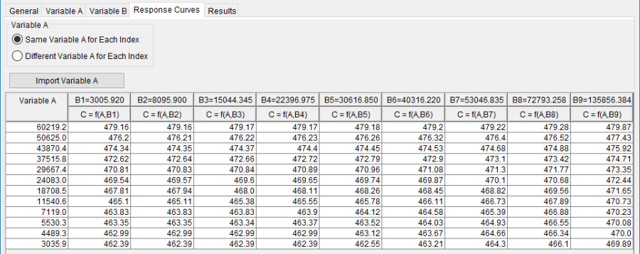
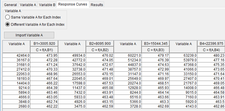
As shown in Figure 1, there are two options for the Response Curves table; Same Variable A for each index or Different Variable A for each index. When the Same Variable A for each index option is selected, there is only one Variable A column in the response curves table. The user can manually fill in the values for Variable A or press the Import Variable A button. When the button is pressed, the program will import the values on the Variable A tab. The user can edit the Variable A values after they are imported. When the Different Variable A for each index option is selected, there is a separate Variable A column for each variable B index value, as shown in Figure 2. The user can manually fill in the values for Variable A or press the Import Variable A button. When the button is pressed, the program will import the values from the Variable A tab. The user can edit the Variable A values after they are imported. In most cases, the Different Variable A for each index options will be used when performing a conditional analysis (variables A and B can not be assumed independent). In this case, a separated variable A frequency curve was defined for each variable B index value; therefore, when the Import Variable A button is pressed the program will import the corresponding frequency curve into the response curves table.
The user must compute the variable C value given the combinations of variables A and B. Figure 1 contains 12 values of variable A and 9 index values for variable B. Therefore, the user would have 108 combinations of variables A and B to compute values of variable C. Once computed, the user would manually enter the variable C values into the response curves table. For example, the first value in the first variable C column in Figure 1 is 481.38. This was computed using a variable A value of 66039 and a variable B value of 3005.92


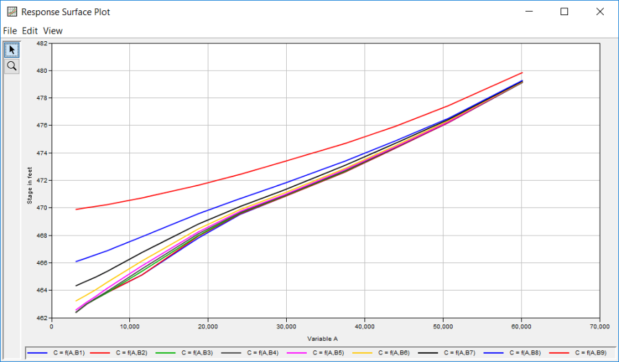
The Plot Response Surface button will open a plot similar to the one shown in Figure 3. Each line in the response surface plot shows the variable C versus variable A relationship for a given variable B index value.
