Download PDF
Download page General Settings for Correlation Analysis.
General Settings for Correlation Analysis
Once the analysis name has been entered, the user can begin defining the analysis. Contained on the Correlation Analysis editor are three tabs. The tabs are labeled General, Location Information, and Results. The first tab contains general settings for performing the Correlation Analysis. These settings include:
- Computation Method
- Number of Locations
- Locations
- Plotting Position
- Output Frequency Ordinates
- Time Window Modification
Computation Method
This option lets the user choose which computational method will be used as shown in Figure 1. Three computational methods are available including Coincident Events (which compares the input data to ensure that they correspond to the same “event”), Coincident in Time (which compares a designated "Primary" data set against "Secondary" data in order to extract values for comparison), and Paired Data (which uses the data as defined by the user without any modifications).

Time Series | Coincident Events
When using this method, pairs of data will be extracted using defined time windows. Time windows must be defined for each location within the Location Information tab. Figure 2 demonstrates how time series will be evaluated when using the Time Series | Coincident Events computational method.
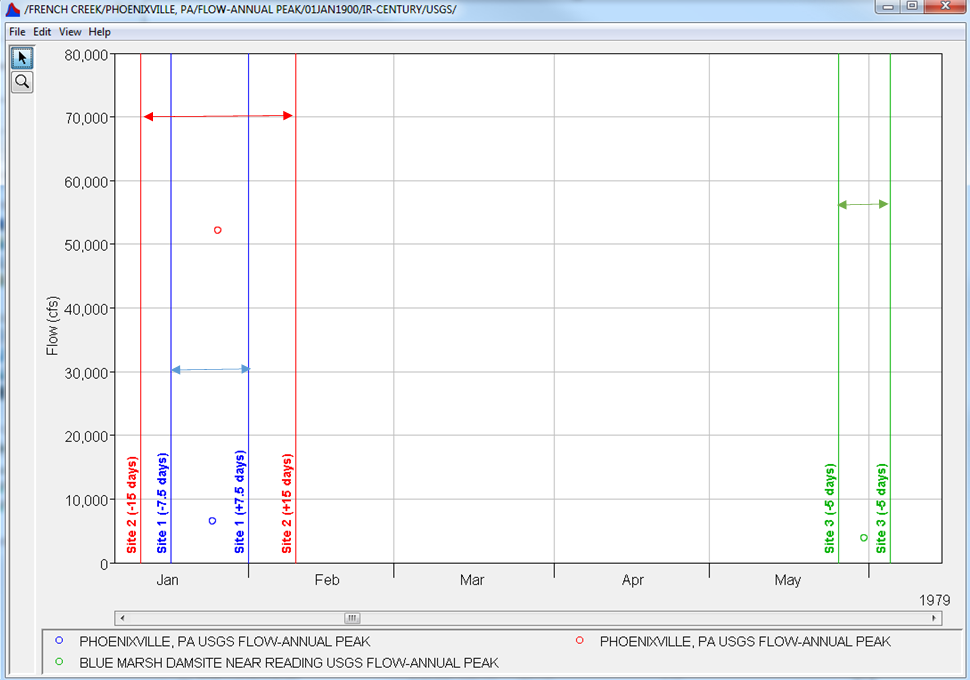
An example application using this computational method can be found here: Coincident Events - West Branch Susquehanna River.
Time Series | Coincident in Time
When using this method, values from the secondary data set(s) will be extracted at the same time as each value within the primary data set. For instance, if the Primary data set has values at 09Dec1972 24:00, 03Mar1972 24:00, 23Mar1972, 24:00, and 17Apr1972, 24:00, values will be extracted from the Secondary data set(s) at those four date-times and used to compute correlation coefficients. Figure 3 demonstrates how time series will be evaluated when using the Time Series | Coincident in Time computational method.
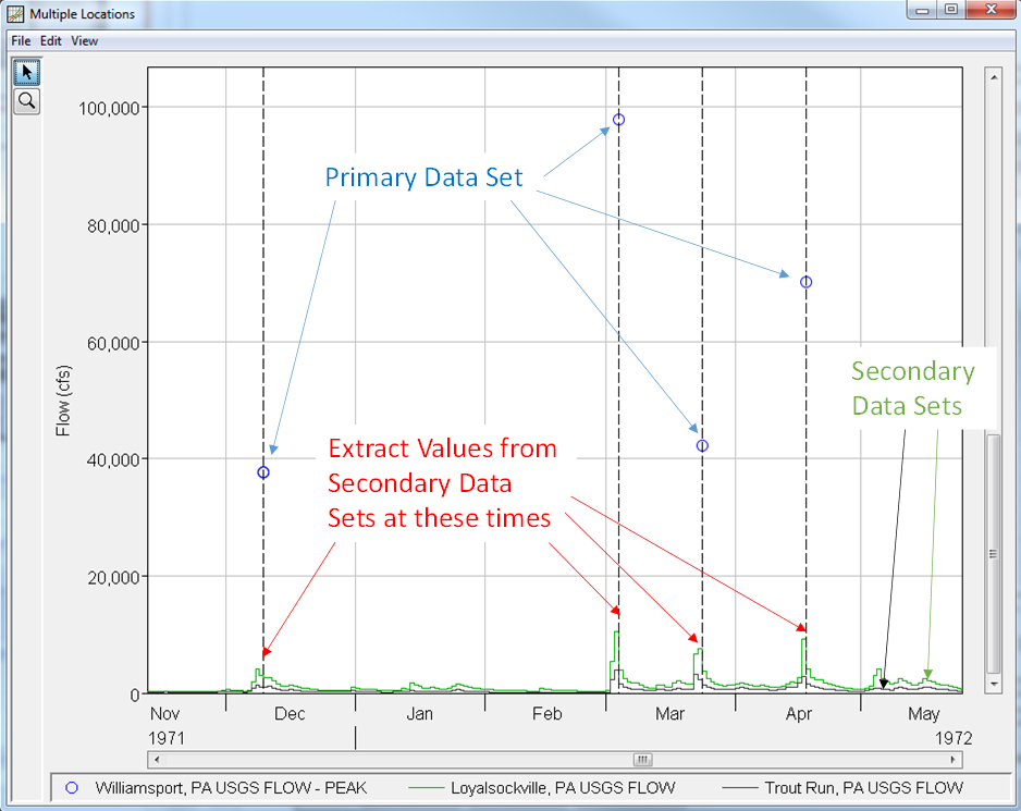
An example application using this computational method can be found here: Coincident in Time - Tar River.
Paired Data
This computational method can be used to determine how closely related the values within paired data curves (i.e. curves with no date/time axis) are with one another. Time windows will not be evaluated when using this method.
An example application using this computational method can be found here: Paired Data.
Number of Locations
This option lets the user choose the number of locations that will be used to compute correlation coefficients as shown in Figure 4. The Location Information tab will update based on the number of curves specified in this panel.
![]()
Locations
This panel allows the user to define an optional Name and select a time series (if using one of the Time Series computational methods) or paired data (if using the Paired Data computational method). When using the Time Series | Coincident Events computational option, this panel will resemble Figure 5.

When the Plot All Time Series button is pressed, all time series will be plotted in the same dialog, as shown in Figure 6.

Plotting Position
Plotting positions are used for plotting the original and/or processed data set on a probability scale. There are four options for computing plotting positions within the Distribution Fitting Analysis as shown in Figure 7: Weibull, Median, Hazen, and user entered coefficients. The default method within the Distribution Fitting Analysis is the Median plotting position formula.

The generalized plotting position equation is:
P=\frac{(m-A)}{(n+1-A-B)}
where: m= rank of flood values with the largest equal to 1.
n= number of flood peaks in the data set.
A & B= constants dependent on which equation is used (Weibull A and B = 0; Median A and B = 0.3; and Hazen A and B = 0.5).
Plotting positions represent estimates of the exceedance (or non-exceedance) probability of each data point. The probabilities of the highest and lowest points in the data set are the most sensitive to choice of plotting position estimator. When fitting an analytical distribution, the plotting of data on the graph by a plotting position method is only done as a guide to assist in evaluating the computed curve. The plotting position method selected does not have any impact on the computed curve.
Output Frequency Ordinates
This option allows the user to change or add to the frequency ordinates for which the resulting frequency curve and confidence limits are computed, as shown in Figure 8. The default values listed in percent chance exceedance are 0.2, 0.5, 1, 2, 5, 10, 20, 50, 80, 90, 95, and 99. Check the box next to Use Values from Table below to change or add additional values. Once this box is checked, the user can add/remove rows and edit the frequency values. To add or remove a row from the table, select the row(s), place the mouse over the highlighted row(s) and click the right mouse button. The shortcut menu contains options to Insert Row(s), Append a Row, and Delete Row(s). The program will use the default values, even if they are not contained in the table, when the Use Values from Table below option is not checked. Finally, all values in the table must be between 0 and 100. Note that these values have no impact on the computed frequency curve, but rather only the values of the curve that are reported.

Time Window Modification
This option, as shown in Figure 9, allows the user to narrow the time window used for the analysis. The default is to use all of the data contained in the selected data sets. The user can enter either a start date for the analysis, an end date, or both a start and end date. If a start and/or end date are used, they must be dates that are encompassed within the data stored in the selected data sets.
