Once the analysis name and data set are selected, the user can begin defining the analysis. Contained on the General Frequency Analysis editor are four tabs. The tabs are labeled General, Options, Analytical, and Graphical. This section of the manual explains the use of the General and Options tabs.

General Settings

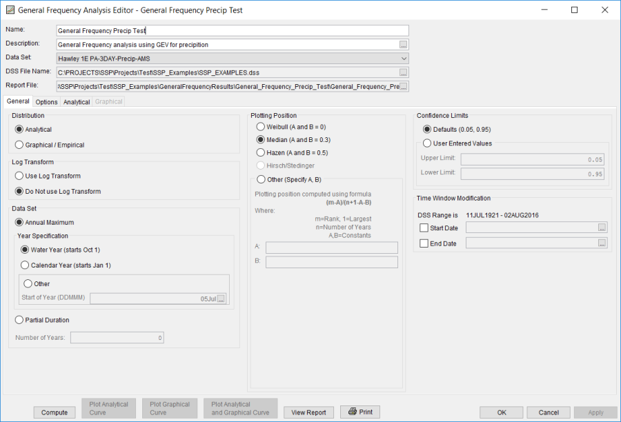
The first tab contains general settings for performing the frequency analysis (Figure 1). These settings include:

• Distribution
• Log Transform
• Data Set
• Plotting Positions
• Confidence Limits
• Time Window Modification

Distribution

There are two options contained within the Distribution setting as shown in Figure 2: Analytical and Graphical / Empirical. If the user selects Analytical, an analytical distribution will be fit to the data when computed. Data and options will need to be selected on the Analytical tab. If the user selects Graphical / Empirical, an empirical distribution will be fit to the data using graphical techniques. Data and options will need to be provided and selected on the Graphical tab. The default setting is Analytical.

Log Transform

There are two options contained within the Log Transform setting as shown in Figure 3: Use Log Transform and Do not use Log Transform. If the user selects Use Log Transform then the logarithms (base 10) of the data will be taken before any computations. If the user selects Do not use Log Transform, then the frequency analysis will be performed on the untransformed data values. The default setting is Use Log Transform.

Data Set

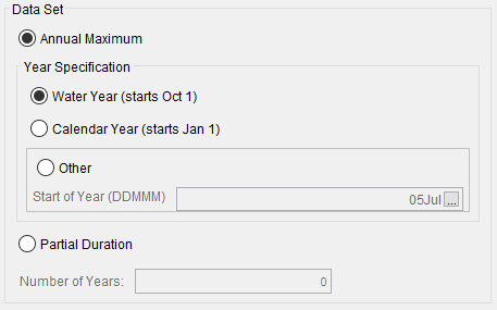
Two methods are available for specifying data within a General Frequency Analysis as shown in Figure 4: Annual Maximum and Partial Duration. Annual Maximum is the default.

An annual maximum series is ordinarily used when the primary interest lies in the larger events or when the second, third, fourth… n^th largest event in any year is of little concern in the analysis. Conversely, a partial duration series represents the frequency of all independent events of interest, regardless of whether two or more occurred in the same year. Partial duration analyses may be more appropriate for situations where considerable flood damage is wrought by the second or third largest flood events in a given year. However, a flow-frequency curve based upon an annual maximum and a partial duration series will converge to form a single flow frequency curve as exceedance probability decreases. Commonly, this convergence occurs between the 0.1 and 0.02 (i.e. 1/10 and 1/50) annual exceedance probabilities.

Peak flow data is most often represented by an annual maximum series. For instance, choosing to download annual peak data from the USGS website (as is detailed here) will result in the import of an annual maximum series. The user is required to produce an appropriate partial duration series for use in a partial duration analysis. This can be achieved in one of several ways. For instance, the user can manually import independent peaks that have been extracted from another data set. However, it is more expedient to use the data filtering options within HEC-SSP, as discussed within the Filtering Data section. Figure 5 demonstrates the differences between a daily average flow data set, an annual maximum series, and a partial duration series for a four year span at a particular stream gage.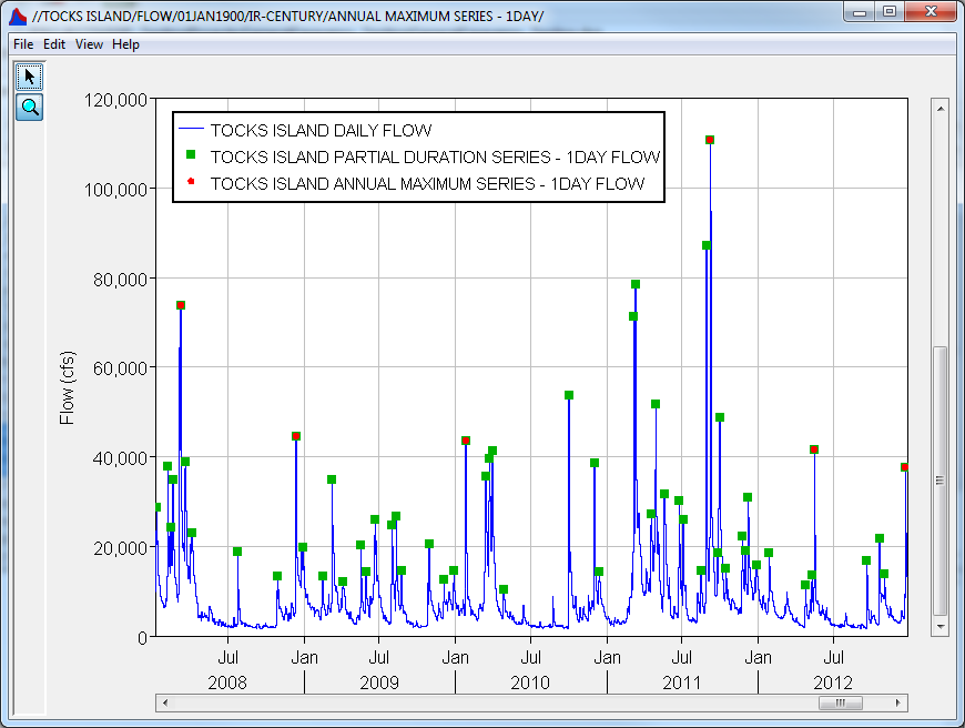

The Year Specification option allows the user to define the beginning and ending date for what will be considered as the analysis year for extracting the data. These dates are used for extracting the annual maxima from the associated data set. It is important to choose a start date that captures all flood events from a certain hydrologic regime. For instance, if high flows generally occur between November and May, then the year should not start between these months. This will minimize the possibility that the same flood event is used for consecutive years. There are three options contained in the Year Specification panel. If Water Year is selected, the program uses a starting date of October 1 and an ending date of September 30. If Calendar Year is selected, the program uses a starting date of January 1 and an ending date of December 31. The Other option lets the user define the starting date. The default is Water Year.

When using a Partial Duration series, the value entered within the Number of Years entry field is used to extract ranked data points from the associated data set. For instance, if the Number of Years is set to 50, then the top 50 ranked events will be extracted from the associated data set regardless of how many years is spanned by the partial duration series.

Plotting Positions

Plotting positions are used for plotting the input data set on a probability scale along with the computed frequency curve and (optional) confidence limits. There are five options for computing plotting positions within HEC-SSP as seen in Figure 6: Weibull, Median, Hazen, Hirsch/Stedinger, and user entered coefficients.

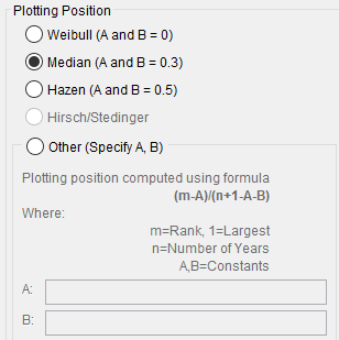
The default method when using an Analytical distribution is the Median plotting position formula. The default method available for computing plotting positions when using the 17C EMA method is Hirsch/Stedinger. The default method when using the Graphical / Empirical distribution is the Weibull plotting position formula. The Hirsch/Stedinger option is only available for use with the 17C EMA method. However, the user may change the plotting position to any they would like and are available for the selected computation options. When using the Hirsch/Stedinger method, the A and B coefficients will be set equal to zero. When using 17C EMA methods and the Hirsch/Stedinger plotting position formula, flow data screened as low outliers (a.k.a. Potentially Influential Low Floods) are assigned a plotting position using the Median plotting position formula within HEC-SSP.

The generalized plotting position equation is:
$//<![CDATA[ \begin{array}{l}P=\frac{(m-A)}{(n+1-A-B)}\end{array} //]]>$
where: m= rank of flood values with the largest equal to 1.
n= number of flood peaks in the data set.
A & B= constants dependent on which equation is used (Weibull A and B=0; Median A and B = 0.3; and Hazen A and B=0.5).

Plotting positions represent estimates of the exceedance probability of each data point (peak flow). Different plotting position formulas can give very different values for the probabilities of the highest and lowest points in the data set. When fitting an analytical distribution, the plotting of data on the graph by a plotting position method is only done as a guide to assist in evaluating the computed curve. The plotting position method selected does not have any impact on the computed curve.

Confidence Limits

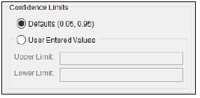
The computed flow frequency curve is only an estimate of the probability distribution of the larger parent population. Confidence limits can be used to provide a measure of the uncertainty of the estimated exceedance probability of a selected discharge, stage, precipitation depth, etc or a measure of the uncertainty of the discharge, stage, precipitation depth, etc at a selected exceedance probability. By default, HEC-SSP calculates the 90 percent confidence interval for all flow frequency analyses (i.e. the 5% and 95% confidence limits). The confidence limits must be entered in decimal form (i.e. 95% = 0.95, and 5% = 0.05). The user has the option to override the default values and enter whatever values they would like for the confidence limits (Figure 7).

Time Window Modification

This option, shown in Figure 8, allows the user to narrow the time window used for the analysis. The default is to use all of the data contained in the selected data set. The user can enter either a start date for the analysis, and end date, or both a start and end date. If a start and/or end date are used, they must be dates that are encompassed within the data stored in the selected data set. The date range for the selected data set is shown in the editor just above the Start Date field.

Any dates entered within the Time Window Modification will be ignored when using the 17C EMA methods. When using 17C EMA, changes to the start and end period should be made within the EMA Data tab.

Options

In addition to the general settings, there are also several options available to the user for modifying the computations of the frequency curves. These options include:

• Low Outlier Threshold
• Output Labeling
• Historic Period Data
• Output Frequency Ordinates

When the Options tab is selected, the General Frequency Analysis editor will appear as shown in Figure 9.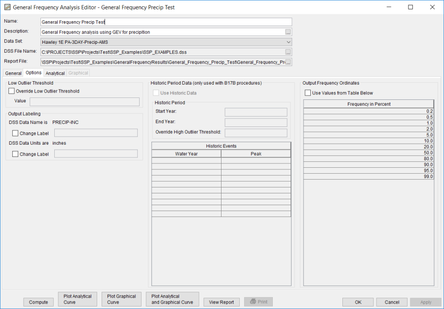

Low Outlier Threshold

The user has the option to enter a different value for the low outlier threshold, if desired. If a value is entered for the low outlier threshold, then this value will override the computed value from either the Single or Multiple Grubbs-Beck test. An error message will be shown if the low outlier threshold is set to a value that would censor more than 50 percent of the values within the data set. To override the computed low outlier threshold, check the box labeled Override Low Outlier Threshold, as shown in Figure 10, and enter the preferred value.

The user may also use this option to screen low outliers when not using either 17B or 17C EMA procedures. However, this option is only available when using analytical distributions. All values less than the user-entered value will then be censored during the computations.

Output Labeling

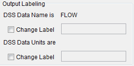
This option, shown in Figure 11, allows the user to change the default labels for data contained in the output tables and plots. The user can change both the name of the data as well as how the units of the data are labeled.

Historic Period Data

All historic data that provides reliable estimates of flood peaks outside the systematic record should be used in order to improve the estimated flood frequency curve. Flood information of large events outside of the systematic record can often be used to extend the record to a historic period much longer than that of the systematic record. HEC-SSP uses historic data specified in this table (Figure 12) as recommended in Bulletin 17B.

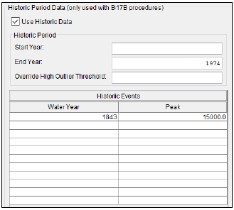
This option is only available when using Bulletin 17B procedures. To make use of historic data within the 17C EMA procedures, this information should be entered on the EMA Data tab. To use historic data with Bulletin 17B procedures, check the box labeled Use Historic Data. The user can enter a starting year for the historic period, ending year for a historic period, and a high threshold value. If the user enters a high threshold value, then any value in the systematic record greater than that value will also be treated as a historical flood peak. The user can also enter historic flood peaks that are not contained in the systematic record. This is done in the table at the bottom labeled Historic Flood Peaks. Only one value per water year may be entered and all years must be entered assuming a water year from October 1 through September 30. If a start year is not entered, then the assumed start year is the earliest year of the systematic record and any historical values that have been entered. If an end year is not entered, then the assumed end year is the latest year in the systematic record and any entered historic values.

Note: The program treats all data in the data set as systematic data when using 17B procedures. If historic events are included in the data set, then the user must define the analysis time window (General tab – Time Window Modification) so that it only bounds the systematic record. Then the user must define the historic events in the Historic Events table.

Output Frequency Ordinates

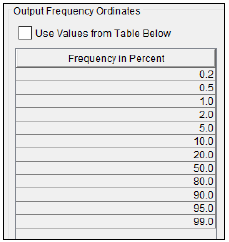
This option (Figure 13) allows the user to change or add to the frequency ordinates for which the resulting frequency curve and confidence limits are computed. The default values listed in percent chance exceedance are 0.2, 0.5, 1, 2, 5, 10, 20, 50, 80, 90, 95, and 99. Check the box next to Use Values from Table below to change or add additional values. Once this box is checked, the user can add/remove rows and edit the frequency values. To add or remove a row from the table, select the row(s), place the mouse over the highlighted row(s) and click the right mouse button. The shortcut menu contains options to Insert Row(s), Append a Row, and Delete Row(s). The program will use the default values, even if they are not contained in the table, when the Use Values from Table below option is not checked. Finally, all values in the table must be between 0 and 100. Note that these values have no impact on the computed frequency curve, but rather only the values of the curve that are reported.