Once the analysis name and data set are selected, the user can begin defining the analysis. Five tabs are contained on the Volume Frequency Analysis editor. The tabs are labeled General, Options, Duration Table, Analytical, and Graphical. This section of the manual explains the use of the General and Options tabs.

General Settings

The first tab contains general settings for performing the frequency analysis (Figure 1).

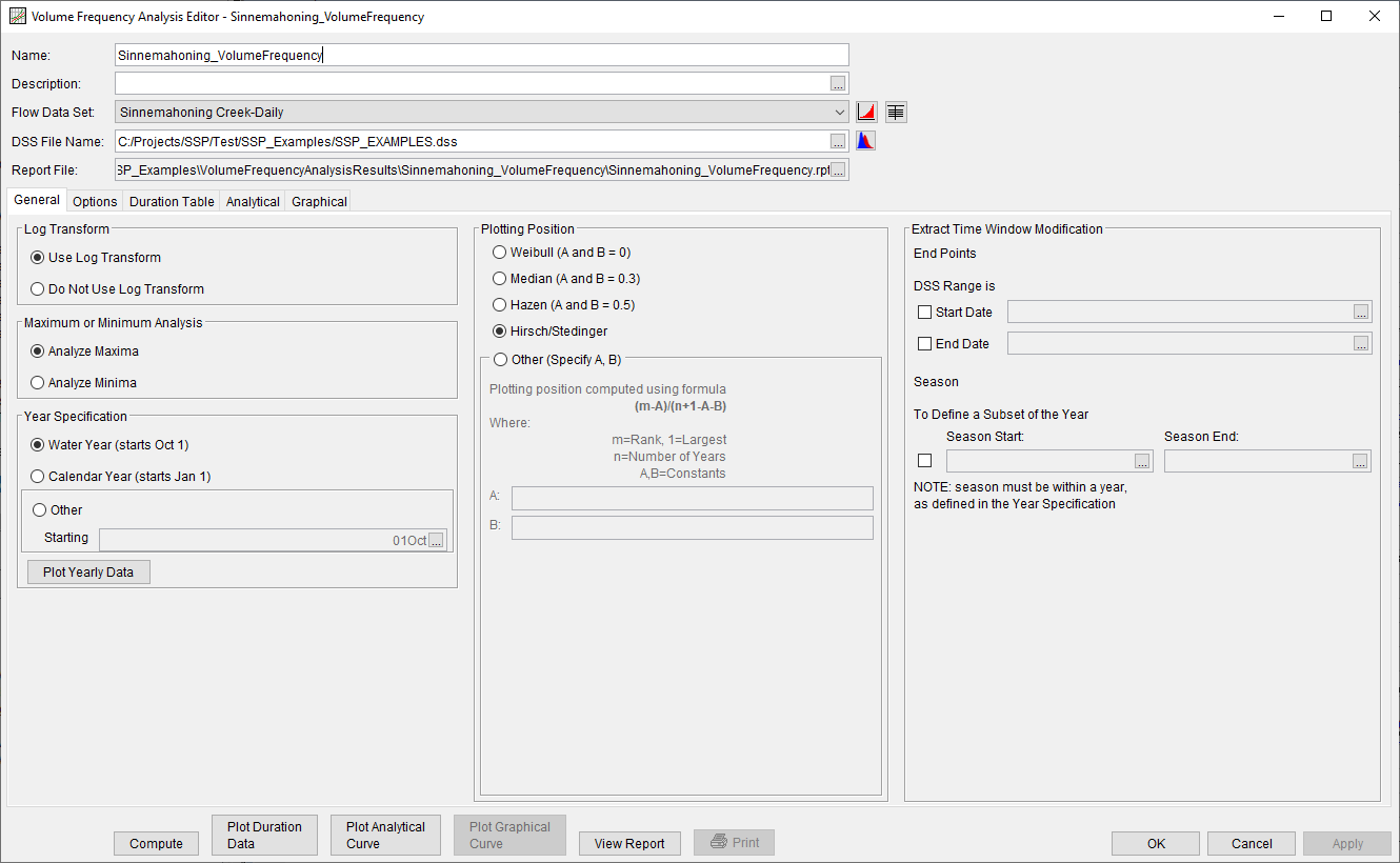
These settings include:

• Log Transform
• Maximum or Minimum Analysis
• Year Specification
• Plotting Positions
• Time Window Modification

Log Transform

There are two options contained within the Log Transform panel, as seen in Figure 2: Use Log Transform and Do not use Log Transform. If the user selects Use Log Transform, then the logs of the data will be computed first, and the frequency analysis will be performed on the logs of the data. If the user selects Do not use Log Transform, then the frequency analysis will be performed on the raw data values without taking the logs of the data. The default setting is Use Log Transform.

Plotting Positions

Plotting positions are used for plotting the input data set on a probability scale along with the computed frequency curve and (optional) confidence limits. There are five options for computing plotting positions within HEC-SSP, as seen in Figure 3: Weibull, Median, Hazen, Hirsch/Stedinger, and user entered coefficients.

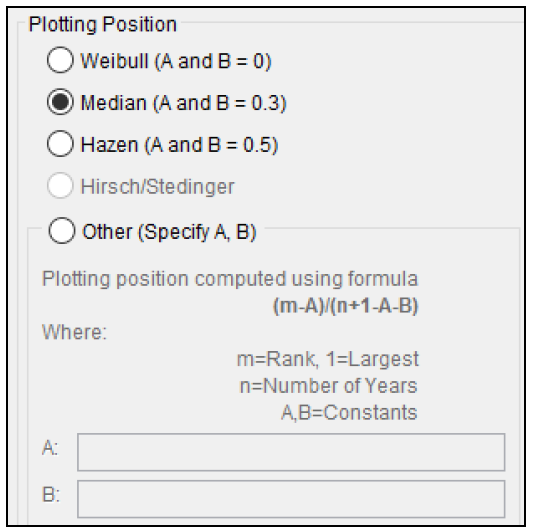
The default method when an analytical distribution is selected is the Median plotting position formula. The default method for computing plotting positions when using the 17C EMA method is Hirsch/Stedinger. The Hirsch/Stedinger option is only available for use with the 17C EMA method. However, the user may change the plotting position to any they would like and are available for the selected computation options. When using the Hirsch/Stedinger method, the A and B coefficients will be set equal to zero. When using 17C EMA methods and the Hirsch/Stedinger plotting position formula, flow data screened as low outliers (a.k.a. Potentially Influential Low Floods) are assigned a plotting position using the Median plotting position formula within HEC-SSP.

The generalized plotting position equation is:

$//<![CDATA[ \begin{array}{l}P=\frac{(m-A)}{(n+1-A-B)}\end{array} //]]>$

where:

m= rank of flood values with the largest equal to 1.
n= number of flood peaks in the data set.
A & B= constants dependent on which equation is used (Weibull A and B=0; Median A and B = 0.3; and Hazen A and B=0.5).

Plotting positions represent estimates of the exceedance probability of each data point (peak flow). Different plotting position formulas can give very different values for the probabilities of the highest and lowest points in the data set. When fitting an analytical distribution, the plotting of data on the graph by a plotting position method is only done as a guide to assist in evaluating the computed curve. The plotting position method selected does not have any impact on the computed curve.

Maximum or Minimum Analysis

A volume frequency analysis can be performed using annual maxima or minima. There are two options contained in the Maximum or Minimum Analysis panel (Figure 4). If Analyze Maxima is selected, then the program will extract annual maximum volumes for each year for each duration. Conversely, if Analyze Minima is selected, then the program will extract annual minimum volumes for each year for each duration.

A flow analysis that analyzes annual maxima could be used for determining the amount of reservoir storage required for a flood of specific frequency. Conversely, an analysis that analyzes annual minima could be used determine if a river could supply a given demand. A low flow analysis could also be beneficial for water quality and reservoir storage projects.

Year Specification

This option allows the user to define the beginning and ending date for what will be considered as the analysis year for extracting the data. These dates are used for extracting the annual maxima or minima in order to get one value for each analysis year. It is important to choose a start date that captures all flood events from a certain hydrologic regime. If high flows generally occur between November and May, then the year should not start between these months. This will minimize the possibility that the same flood event is used for consecutive years.

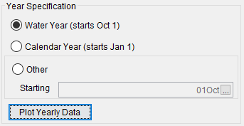
There are three options contained in the Year Specification section, as seen on Figure 5. If Water Year is selected, the program uses a starting date of October 1 and an ending date of September 30. If Calendar Year is selected, the program uses a starting date of January 1 and an ending date of December 31. The Other option lets the user define the starting date. The default is Water Year.

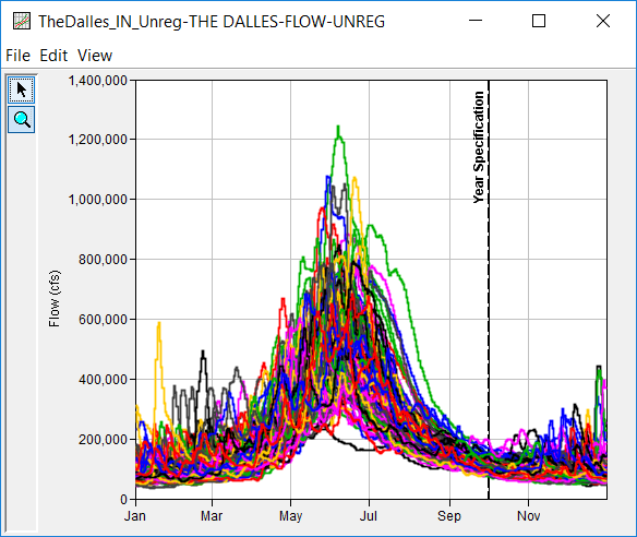
When the Plot Yearly Data button is pressed, a graph will be created that overlaps the flows for each year on a common x-axis that spans January 1^st to December 31^st. A vertical, dashed line will be placed at the specified Year Specification date. This plot can be useful when determining the Year Specification date that is most appropriate for the desired analysis. The flows shown in Figure 6 are from a location that experiences snowmelt and occasional rain-on-snow floods. Starting the year on October 1 when analyzing annual maxima is appropriate for this data set since no large floods occur near that date. Conversely, if annual minima of are interest, a Year Specification Date of June 15^th may be the most appropriate since no low flows occur near that date.

Time Window Modification

This option allows the user to narrow the time window used for the analysis (Figure 7). When left unchecked, the program will use all of the data contained in the selected data set. The user can enter either a start or end date or both a start and end date. If a start and/or end date are used, they must be dates that are included within the selected data set. The date range for the selected data set is shown in the editor just above the Start Date field.

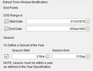
An additional option at the bottom of the time window modification panel allows the user to define a shorter duration (i.e. a Season) within the year in which the program extracts maxima or minima. This option allows the user to analyze events that typically occur during a specific season, like snowmelt floods. When left unchecked, the program will examine all flow records during the year. The season start and end dates must be entered using a two digit day followed by the month (i.e. 15May). The season start and end dates must fall within a year as defined in the Year Specification. The user must enter both start and end dates to define the season subset.

Options

In addition to the general settings, there are also several options available to the user for modifying the computation of the volume-frequency curves. These options include:

• Flow Durations
• Output Labeling
• Output Frequency Ordinates
• Low Outlier Threshold
• Historic Period Data

When the Options tab is selected, the Volume Frequency Analysis editor will appear as shown in Figure 8.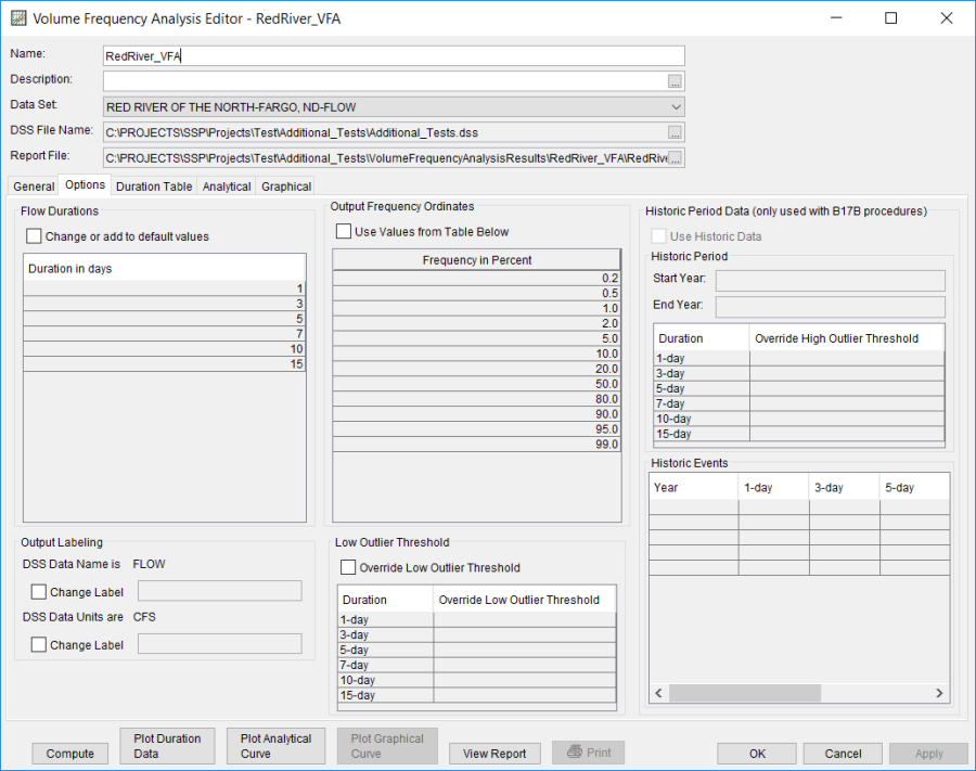

Flow-Durations

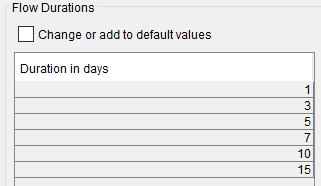
This option, shown in Figure 9, lets the user define which durations are used in the volume frequency analysis. The program will extract annual maximum or minimum volumes for each year for each duration based on the durations defined in this table. The default durations are 1-, 3-, 5-, 7-, 10-, and 15-days. Check the box next to Change or add to default values to change or add additional durations to the analysis. Once this box is checked, the user can add/remove rows and/or edit the duration values. To add or remove a row from the table, select the row(s), place the mouse over the highlighted row(s) and click the right mouse button. The shortcut menu contains options to Insert Row(s) and Delete Row(s). The program will use the default durations, even if they are not contained in the table, when the Change or add to default values option is not checked.

Output Frequency Ordinates

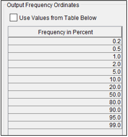
This option (Figure 10) allows the user to change or add to the frequency ordinates for which the resulting frequency curve and confidence limits are computed. The default values listed in percent chance exceedance are 0.2, 0.5, 1, 2, 5, 10, 20, 50, 80, 90, 95, and 99. Check the box next to Use Values from Table below to change or add additional values. Once this box is checked, the user can add/remove rows and edit the frequency values. To add or remove a row from the table, select the row(s), place the mouse over the highlighted row(s) and click the right mouse button. The shortcut menu contains options to Insert Row(s), Append a Row, and Delete Row(s). The program will use the default values, even if they are not contained in the table, when the Use Values from Table below option is not checked. Finally, all values in the table must be between 0 and 100. Note that these values have no impact on the computed frequency curve, but rather only the values of the curve that are reported.

Output Labeling

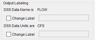
This option (Figure 11) allows the user to change the default labels for data contained in the output tables and plots. The user can change both the name of the data and how the units of the data are labeled.

Low Outlier Threshold

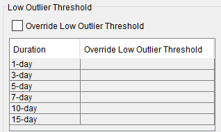
The user has the option to enter a different value for the low outlier threshold, if desired. If a value is entered for the low outlier threshold, then this value will override the computed value from either the Single or Multiple Grubbs-Beck test. An error message will be shown if the low outlier threshold is set to a value that would censor more than 50 percent of the values within the data set. To override the computed low outlier threshold, check the box labeled Override Low Outlier Threshold, shown in Figure 12, and enter the preferred value. The user may also use this option to screen low outliers when not using either 17B or 17C EMA procedures. All values less than the user-entered value will then be censored during the computations. To use the low outlier threshold, simply check the box and enter a value for one or more durations.

Historic Period Data

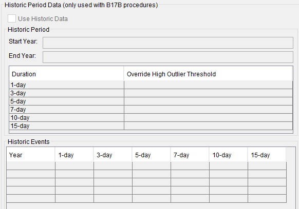
All historic data that provides reliable estimates of flood peaks outside the systematic record should be used in order to improve the estimated flood frequency curve. Flood information of large events outside of the systematic record can often be used to extend the record to a historic period much longer than that of the systematic record. HEC-SSP uses historic data specified in this table as recommended in Bulletin 17B.

This option is only available when using Bulletin 17B procedures, as shown in Figure 13. To make use of historic data within the 17C EMA procedures, this information should be entered on the EMA Data tab. To use historic data with Bulletin 17B procedures, check the box labeled Use Historic Data. The user can enter a starting year for the historic period, ending year for a historic period, and a high threshold value. If the user enters a high threshold value, then any value in the systematic record greater than that value will also be treated as a historical flood peak. The user can also enter historic flood peaks that are not contained in the systematic record. This is done in the table at the bottom labeled Historic Flood Peaks. Only one value per water year may be entered and all years must be entered assuming a water year from October 1 through September 30. If a start year is not entered, then the assumed start year is the earliest year of the systematic record and any historical values that have been entered. If an end year is not entered, then the assumed end year is the latest year in the systematic record and any entered historic values.

Note: The program treats all data in the data set as systematic data when using Bulletin 17B procedures. If historic events are included in the data set, then the user must define the analysis time window (General tab – Time Window Modification) so that it only bounds the systematic record. Then the user must define the historic events in the Historic Events table.