Creating a Stochastic Data Importer Plugin Alternative
This page describes the process to create a new SDI plugin alternative and the functionality of the options in the SDI editor user interface.
Creating the SDI Alternative
Right click on the Stochastic Hydrologic Data Importer from the Models Tree Node of the Study Tree and select New…
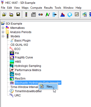
Note that the name "Stochastic Hydrologic Data Importer" is used in this list, an old name that persists here due to backwards compatibility requirements.
This will elicit the Create New SDI Alternative Editor as shown below. Define a name for the alternative and select OK. This name can be changed later in the editor window.

Create New SDI Alternative Editor
The Stochastic Data Import Editor appears as presented below.

Stochastic Data Importer Editor
This SDI Editor window consists of several tabs:
- Events: On this tab, enter information about the dimensions of the data to be brought into the model via the SDI plugin. The length of the analysis period used for the simulation should match the number of years in a lifecycle, and the collection identifiers on the input data should be numbered 1 through the number of lifecycles being computed. The number of realizations and number of years per realization should be consistent with these two dimensions. If the nested Monte Carlo sampling features are used elsewhere, the realization size is used to determine when knowledge uncertainty-linked parameters are resampled, and the length of a lifecycle may have an impact on features where the sequence of events impact the results. If the SDI plugin is being used without the other nested Monte Carlo sampling features in HEC-WAT, the primary thing that will determine the size of the lifecycle and realizations will be the size of the model computes desired. For example, if the SDI plugin is being used to allow computing many RAS models in a distributed compute at once, the number of years per lifecycle and per realization may be 1.
- Locations & Parameters: This tab is used to input the locations and parameters that will be output by the Stochastic Data Importer and made available in the model linking editor.
- DSS information: Once locations and parameters are determined on the previous tab, the DSS filename and pathnames for each location and parameter combinations are entered on this tab.
- Validate: This tab has a single button that validates the input data matches the expected format for the SDI plugin and provides a list of issues if any are found.
Events Tab
This tab has several important settings for configuring the SDI alternative – features that were planned but not currently ready for use are greyed out. The Start of Year section presents three radio buttons for choosing the date that divides the data into distinct events, which may be full years in length. The choices are Water Year, splitting the data on October 1st, Calendar Year, splitting the data on January 1st, or Other allowing a choice of other dates to use. Each year of input data, divided by the date selected, will be run through the HEC-WAT simulation's model sequence as a single event, with Monte Carlo parameters designated as "natural variability" inputs being sampled before each event. This start of year date must match the day of year used for the start of the analysis period.
The inputs Event/Year Count, for Data Check and DSS File Setup has two important functions:
- First is a radio button choice for Start Lifecycles at C:000000 or Start Lifecycles at C:000001, which selects the initial collection ID for the DSS records containing the first lifecycle of data.
- The remaining fields and the table below them are used to enter the dimensions of the data. This is not used at compute time, but by the validation step to confirm that the dimensions of the data in the DSS records match the expected compute size. The number of realizations, years per realization, and years per lifecycle are used to calculate the dimensions of the expected input data. The lifecycles per realiaztion and lifecycles in a simulation are calculated from the inputs, and the table below them is used to show which lifecycles are associated with each realization.
Locations and Parameters Tab
This tab is used to define the locations that are needed to produce data for models below the SDI in the program order. These locations and parameters are made available by the model linking editor, and combinations of each should be added for all inputs expected by the models to be run in the HEC-WAT FRA Simulation. Each location may have one or more parameter selected. The naming of the locations are entered as text, but matching the naming convention of the consuming model (such as HEC-HMS, HEC-ResSim, or HEC-RAS) will simplify the model linking stage later in the workflow. Similarly, naming the input DSS records to match will make it easier to check that inputs are mapped correctly.
In the Creation of Data locations panel, select the New button to add additional locations, Rename to change their name, Save As... to create a copy with a new name, and Delete... to remove them.
For each location added, a series of check boxes in the bottom half of the window allow selecting the parameters for that location. Similarly, New... creates additional parameters, Rename changes the name, and Delete... removes them. A default set of Flow, Precip, and Temp (for precipitation and temperature) are provided, however any parameter may be added, although parameter names cannot match an existing location name.
Once locations are added and parameters selected, the dropdown at the top of the window Location/Parameter Pair as Primary for Event Dates should be used to select one input time series. Presence or absence of data in this time-series will be used to further limit the simulation time window for each event. After splitting the time-series into years using the Start of Year date selected on the prior tab, the first and last valid value in this time-series will be used to determine the start and end of the time window for each event.

DSS Information Tab
This tab provides a table for entering the DSS time-series record name and the source DSS file for each location and parameter created on the Locations & Parameters tab that need DSS paths defined. All data for a single location/parameter pair must be in the same DSS file.
Select the first row and then press the Select DSS Path button in the lower right hand corner. Browse to the project’s shared data folder and select the corresponding DSS file, then choose the DSS record that matches. In the example below, the DSS record selected matches the location name for the B part and the C part corresponds to the "type" or parameter chosen.
From the SDI editor, once a location is selected, one can choose the Plot or Tabulate buttons at the lower left hand corner of the window to view that data.

It is a best practice to move the DSS dataset into the watershed or study directory for the WAT model, typically under the "shared" folder or "sdi" folder, so that the data will always be stored with the WAT project in case the project is shared from one computer to another. Check the shared directory and make sure that the “test.dss” file is there, if not copy the file to the shared directory. At compute time, the SDI will copy data from the source DSS Files to the appropriate lifecycle DSS File of the compute. The data copied will be dependent on the date range of the Analysis Period. To ensure your data is retrieved properly, it is best to make the Analysis Period in the WAT match the DSS data utilized by the SDI.
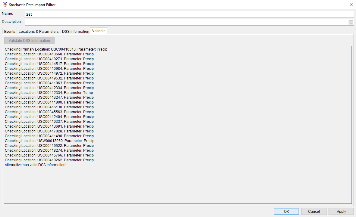
Validate Tab
Once DSS records have been selected, the Validate DSS Information button on this tab can be used to confirm that data is present for all time-series, providing a check that the model compute will not encounter missing data later.