HEC-WAT Setup
HEC-WAT provides the ability to perform the Monte Carlo sampling using the Flood Risk Analysis compute. The FRA compute uses a nested Monte Carlo approach to quantify both knowledge uncertainty and natural variability. Within the Hydrologic Sampler, the precipitation-frequency moments and its associated equivalent record length characterize the outer loop representing knowledge uncertainty. For each realization in this outer loop, a new bootstrapped precipitation-frequency curve is generated. The inner loop captures natural variability by varying storm patterns, areal reduction factors, and HEC-HMS basin model parameters. Each simulation within the inner loop uses a different combination of storm pattern, rainfall depth, areal reduction factor, and basin parameters to reflect inherent hydrologic variability.
The following plugins are used for the FRA analysis. The tasks describe the plugin responsibility for a given realization:
| Plugin | Task |
|---|---|
| Hydrologic Sampler | Sample rainfall depth and storm pattern to create design storm |
| Scripting Plugin | Take sampled design storm from HS and reduce depth by a factor |
| HEC-HMS | Take reduced storm from Scripting Plugin and simulate into rainfall-runoff model. For each simulation, sample a set of basin parameters. |
| Duration | Take flow output from HEC-HMS and compute the 2-day average flow. |
1.Import Models and set up Program Order
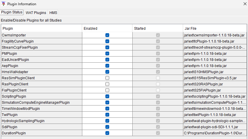
The HEC-HMS model set up for HEC-WAT is imported to HEC-WAT. The Scripting Plugin and Hydrologic Sampler are built into HEC-WAT. The Duration Plugin needs to be downloaded and placed in a directory specified in the HEC-WAT-Personal.config file. Once the Duration Plugin is added, you can head over to Tools | Plugin Information to ensure the Duration Plugin was added correctly.
The HEC-WAT Output Variables for HEC-HMS will only compute the peak value for a selected variable. There is no built-in option within the HEC-WAT to choose a different duration. The Duration Plugin computes a volume average of a given variable (flow, precipitation, etc.) and can be added as an Output Variable to create a volume frequency curve. The Duration Plugin currently lacks a user interface, so its configuration must be done through an XML file generated when the plugin is added to the project. This XML file is stored in the project directory within the DurationPlugin folder. The Duration Plugin is setup to compute the maximum flow volumes for 24-hour, 48-hour, and 72-hour durations.
Duration Plugin needs to be added either in the HEC-WAT.config file or in a HEC-WAT-Personal.config file (placed in C:\Users\"Profile Name"\AppData\Roaming\HEC\HEC-WAT). Place the Duration Plugin jar (unzipped) in the a folder you specify and include the path location in the configuration file.
Download here: DurationPlugin-1.0.zip
Configuration file example: HEC-WAT-Personal.config
Documentation: https://github.com/HydrologicEngineeringCenter/DurationPlugin
Example XML File: example.dp
The Program Order defines the sequence in which models are executed, with models running sequentially. A new Program Order is shown below. Note that HEC-WAT automatically assumes the Hydrologic Sampler runs first, so it does not need to be explicitly specified.
| Setting | Options |
|---|---|
| Program Order |
|
| Analysis Period | 50 years (1/1/2000 - 12/31/2050) |
2. Setup Scripting Plugin
The Scripting Plugin was utilized to apply depth-area reduction factors derived from the HEC-HMS development process. The Scripting Plugin manipulates the output data from one model to be passed as input to another model. More information on Scripting Plugin can be found here. Input and Output locations were added to Data Locations, where the Input receives unreduced rainfall depths from the Hydrologic Sampler, and the Output passes the reduced depths to the HEC-HMS model. The following Jython script reduces the rainfall depth from the storm generated by the Hydrologic Sampler by applying a randomly selected reduction factor.
import random
from com.rma.io import DssFileManagerImpl
from com.rma.io import DssFileManagerImpl
from hec.hecmath import TimeSeriesMath

##
#
# computeAlternative function is called when the ScriptingAlternative is computed.
# Arguments:
#   currentAlternative - the ScriptingAlternative. hec2.wat.plugin.java.impl.scripting.model.ScriptPluginAlt
#   computeOptions     - the compute options.  hec.wat.model.ComputeOptions
#
# return True if the script was successful, False if not.
# no explicit return will be treated as a successful return
#
##
def computeAlternative(currentAlternative, computeOptions):
	output = None
	currentAlternative.addComputeMessage("Computing ScriptingAlternative:" + currentAlternative.getName() )

	for loc in currentAlternative.getInputDataLocations():
		currentAlternative.addComputeMessage(loc.getName())

		# 1. read time series
		tsc = currentAlternative.loadTimeSeries(loc)
		hm = TimeSeriesMath(tsc)

		#2. Choose a reduction factor
		arf = selectArf()

		# 3. multily time series by randomly selected areal reduction factor
		hm = hm.multiply(arf)
		currentAlternative.addComputeMessage("reduced")

		# 4. add to output
		output = hm


	# write output
	dfm = DssFileManagerImpl.getDssFileManager()
	odl = currentAlternative.getOutputDataLocations()[0]
	output.setPathname(odl.getDssPath())
	currentAlternative.writeTimeSeries(output.getData())
	currentAlternative.addComputeMessage("saved output")

	return True

def selectArf():
    numbers = [.87, .813, .824, .904, .919, .903, .842, .915]
    arf = random.choice(numbers)
return arf 3. Setting up Events and Realizations
Similar to the Hydrologic Sampler setup, the modeler must determine an appropriate number of events to simulate per realization. Initial testing, which focused solely on uncertainty in the precipitation-frequency curves, began with 200 events. This starting point was evaluated using both the Hydrologic Sampler and the HEC-HMS model by analyzing the resulting output flow frequency curves. Additional events were then added in increments of 50 to assess whether the output flow frequency curves showed changes to the 1% AEP for a single realization. Even when increasing the number of events to 500, no notable differences in the 1% AEP were observed in the results compared to 200 events. Consequently, 200 events were kept for the Flood Risk Analysis.
The number of realizations was set to 500. A realization refers to a single simulated scenario generated by randomly sampling from the probability distributions of input variables. Each realization represents one possible state of the system under study, capturing the uncertainty in the model parameters. In this modeling context, each realization corresponds to one iteration of the outer loop in the Monte Carlo simulation, reflecting the knowledge uncertainty about the precipitation-frequency curve as represented by its statistical moments. By generating many such realizations, Monte Carlo methods enable estimation of statistical properties—such as means and confidence intervals.
An appropriate number of realizations is generally determined through convergence testing, where a statistical property of interest (e.g., the mean value of the 1% Annual Exceedance Probability [AEP]) stabilizes within a specified tolerance as additional realizations are added. In this analysis, the number of realizations was primarily constrained by compute time considerations. The estimated compute time per event was approximately 2 seconds, so:
For 200 events: 200 × 2 seconds = 400 seconds (~6.7 minutes)
For 500 realizations: 500 × 6.7 minutes = 3,350 minutes (~55.8 hours)
To manage this compute load efficiently, the analysis was split across two computers by dividing the range of realizations. Computer 1 handled realizations 1 through 250. Computer 2 handled realizations 251 through 500. This parallelization effectively halved the compute time per machine to roughly 28 hours.
4. Flood Risk Analysis Simulation
Once the Program Order, Analysis Period, number of Events, and number of Realizations were determined, the Flood Risk Analysis simulation could begin. Output variables included precipitation, peak outflow, 24-hour outflow volume, and 48-hour outflow volume.
Before running the full set of 500 realizations, the model was tested with 10 realizations, and the expected flow volume outputs were compared against the observed expected flow frequency curve at San Lorenzo. Two parameters—constant loss and storage coefficient—were found to have the largest impact on both the peak flow curve and the 2-day volume curve. Instead of sampling from the Parameter Values Sample table for these two parameters, a single value was used for constant loss and storage coefficient and slightly adjusted to better align the simulated results with the 10% Annual Exceedance Probability (AEP) values of the observed peak flow and 2-day volume frequency curves. The remaining basin parameters were varied using the Parameter Value Samples sampling method.
| Parameter | Event Calibration (average) | Continuous Simulation | FRA test |
|---|---|---|---|
| Constant Loss (in/hr) | 0.16 | 0.25 | 0.21 |
| Storage Coefficient (hr) | 3.7 | 6 | 6 |
Once the parameters were set, the full 500 realizations was started. The compute took roughly a total of 80 hours (40 hours per computer).
To combine rainfall-runoff model outputs with peak flow-frequency curves, the rainfall-runoff outputs must be generated independently of the peak flow frequency curve derived from B17C. The constant loss rate and storage coefficient should use the event-based calibration values to maintain this independence.