Results
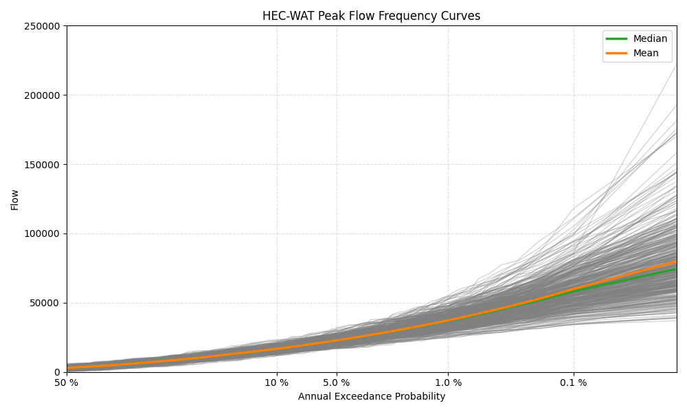
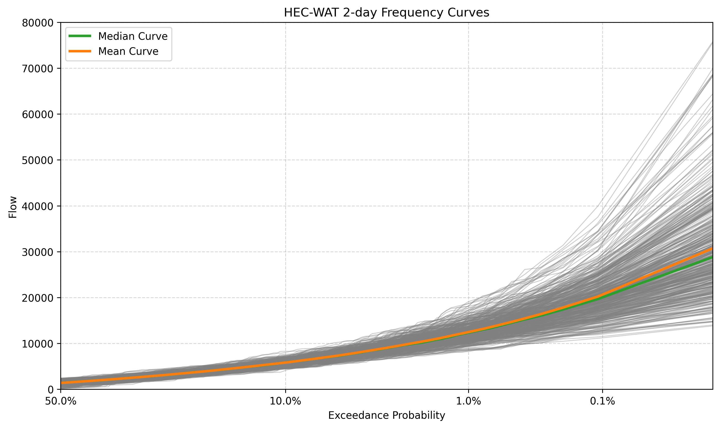
For each realization, an empirical frequency curve is created by determining the incremental probability of the stratified output, ranking the stratified output, and assigning an adjusted plotting position using the Hazen Plotting Position technique. The frequency curve outputs for all saved Output Variables are computed in HEC-WAT and saved in the Realization HEC-DSS file. The plot below shows the peak and 2-day volume frequency curves for all 500 realizations from HEC-HMS.
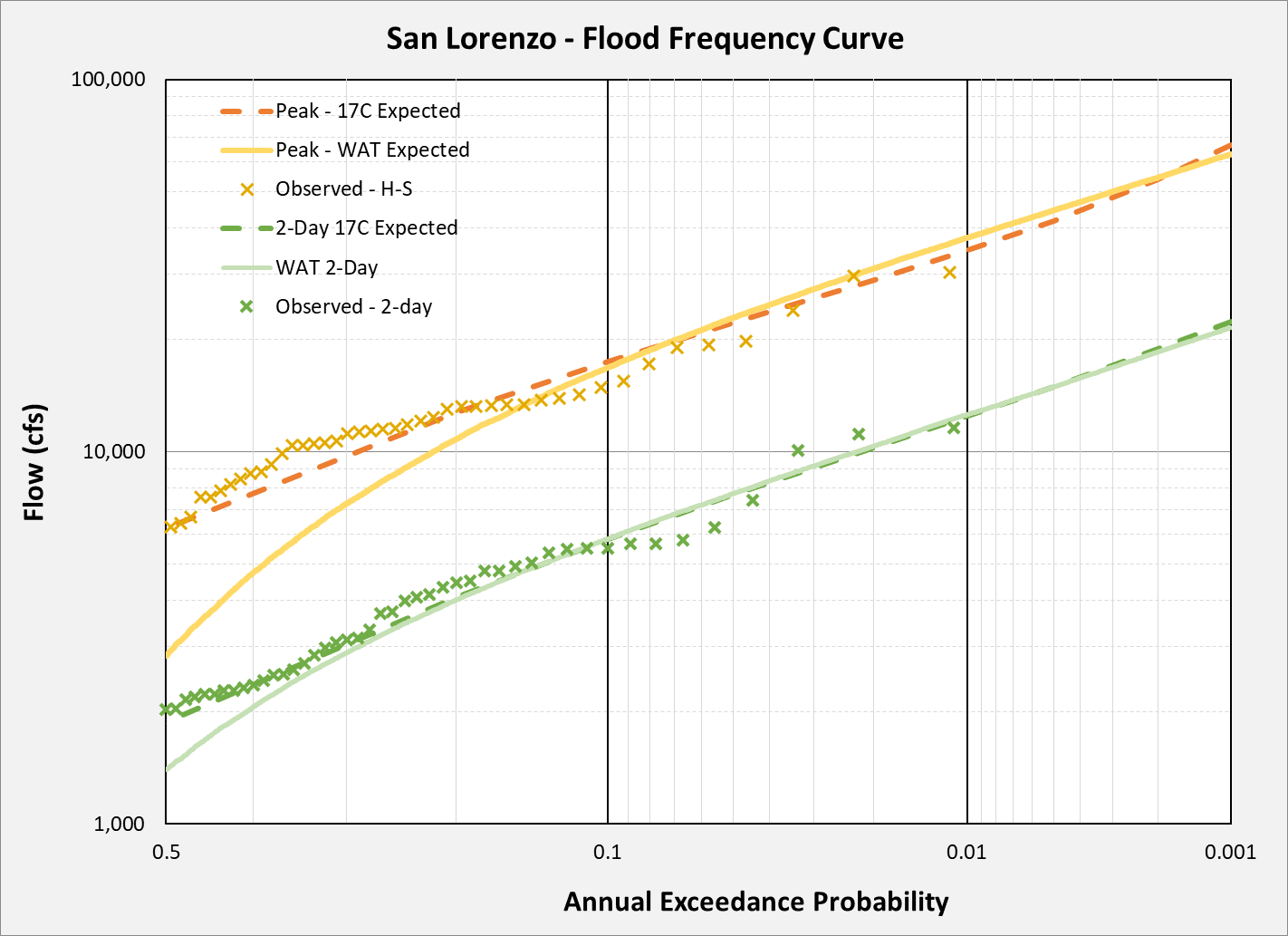
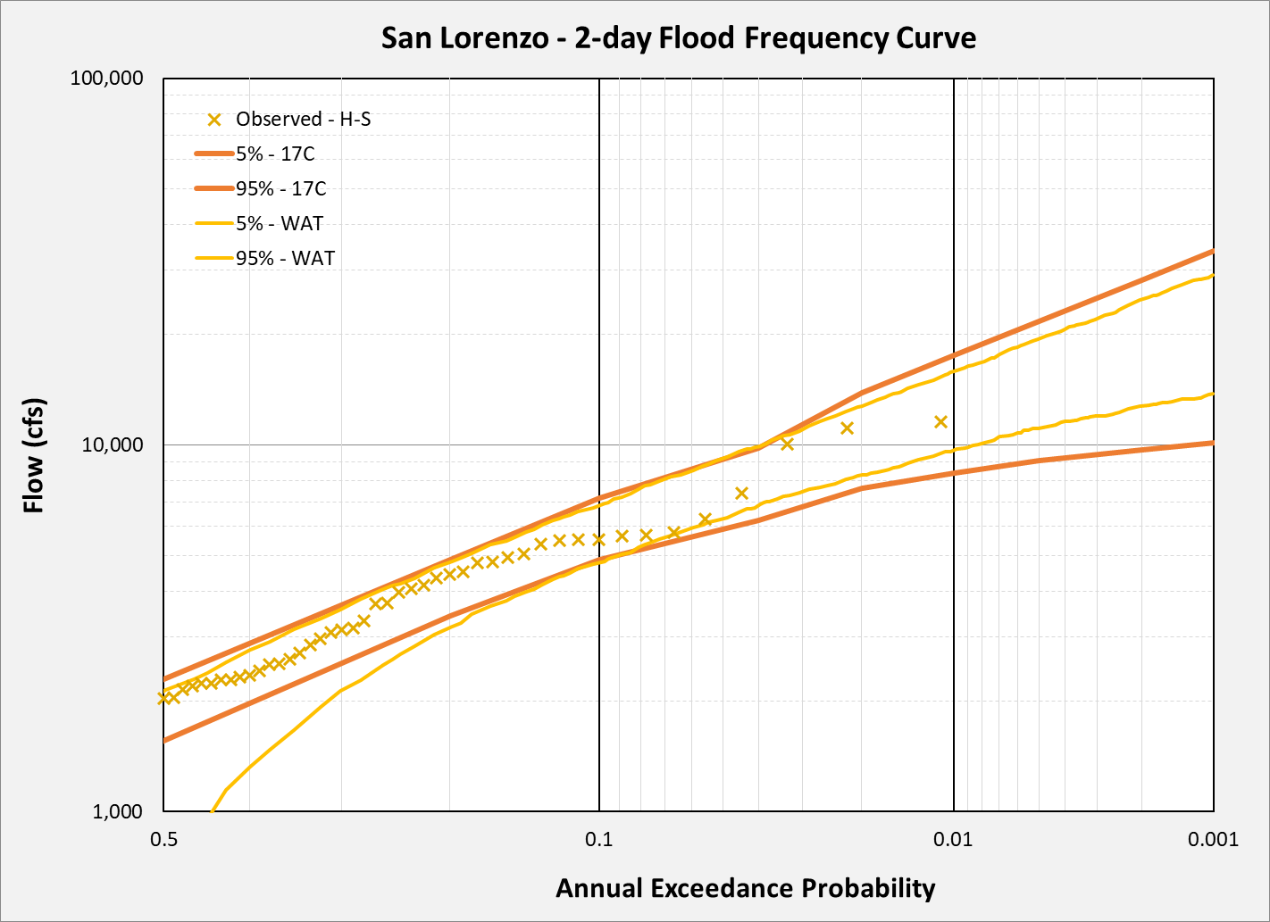
The plot below compares the expected peak and 2-day volume flow frequency derived from Bulletin 17C (B17C) methods, HEC-WAT simulations, and observed peak flows from 1937 to 2021. The peak flows show the HEC-WAT results underestimating the frequency of lower-magnitude peak flows (i.e., those with AEPs greater than 10%), but better aligns with B17C estimates for higher-magnitude events (AEPs less than 10%). This suggests that this HEC-WAT analysis is better adept for simulating extreme flood events than common flows. In contrast, the simulated 2-day volumes from HEC-WAT shows better agreement with B17C estimates across a broader range, specifically from about the 30% AEP down to the 0.1% AEP.
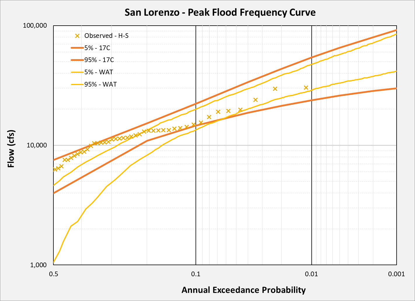
The plot below shows the 5% and 95% confidence interval for peak and the 2-day flow for B17C and HEC-WAT. For the peak flow, the observed data fall within the confidence bounds from the 20% to the 1%. The observed data falls within the confidence bounds for the 2-day volume.
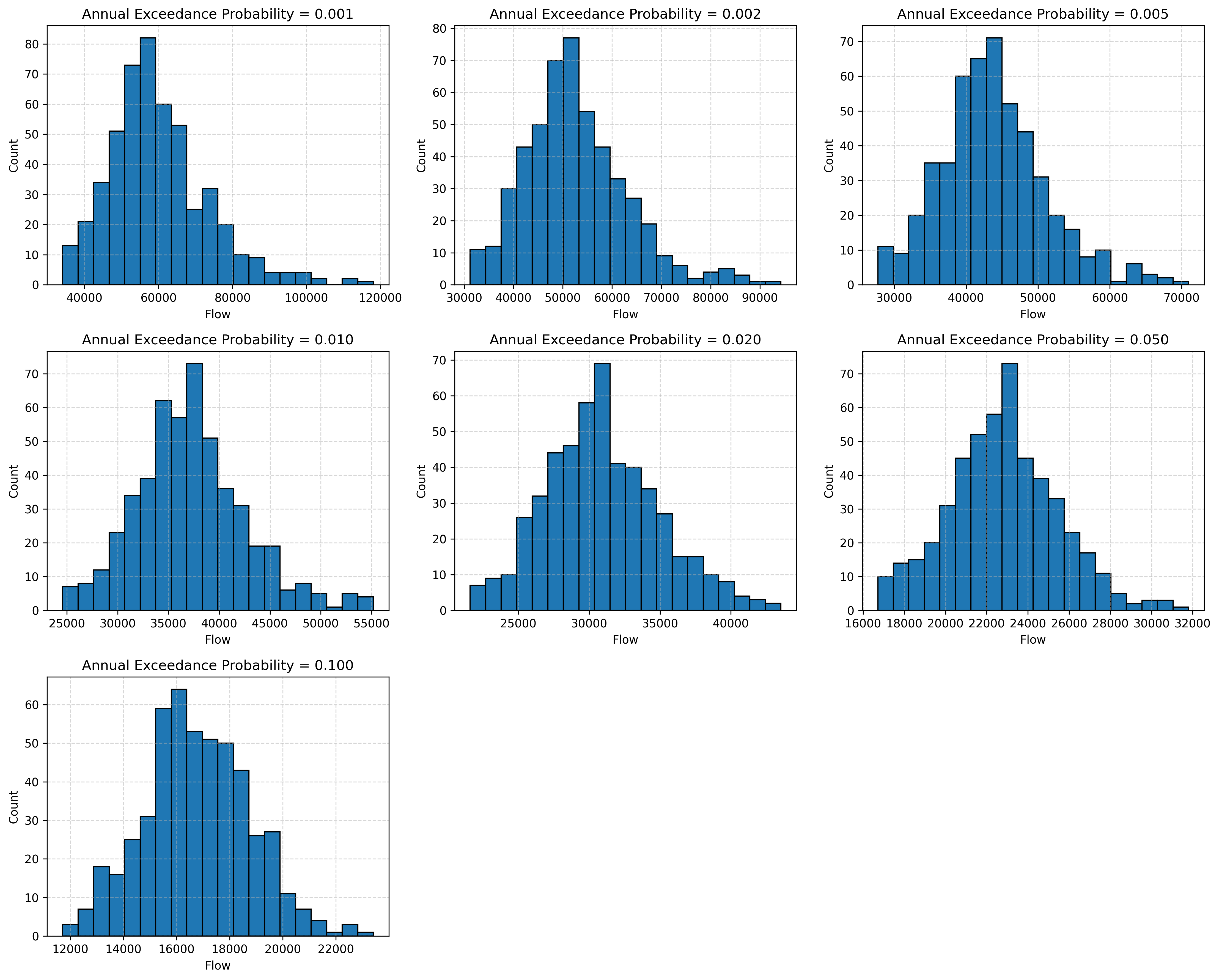
The plot below displays the distribution of flow values for each quantile between 10% and 0.1% AEP, grouped into 20 bins. From 10% to 1% AEP, the histograms appear relatively symmetrical, whereas for lower probabilities (0.5% to 0.1% AEP), the distributions become increasingly right-skewed.
Application
This analysis demonstrates how HEC-WAT can be used to sample from multiple uncertain variables to generate a flow frequency curve that accounts for system variability and provides confidence intervals. The results indicate that the computed frequency curve aligns well with observed data from the 10% to the 0.1% AEP. In this study, two key parameters—constant loss and storage coefficient—were fixed and calibrated to match the observed frequency curve, while the remaining basin parameters were varied using the Parameter Value Sample method. The simulated outputs validate the observed flow frequency quantiles at exceedance levels such as 1% and 0.1% AEP, which are typically challenging to estimate accurately without long-term flow records.
While the San Lorenzo flow gage benefits from over 90 years of peak flow data, many other gages have much shorter records, often limited to 30–40 years or less. When storm and basin parameters are reasonably well characterized through calibration, the range of possible outflows can also be better constrained. This may help reduce (or possibly increase) the uncertainty compared to analyses that rely solely on frequency curves derived from observed flow data, as shown in the results. For these cases, stochastic rainfall-runoff modeling offers a powerful tool for extending flow frequency analyses beyond the available data. By leveraging Monte Carlo sampling within a physically based hydrologic model framework, modelers can incorporate storm and basin parameter variability when estimating rare-event flows (e.g., 1% or 0.2% AEP). This capability is especially valuable for consequential flood risk decisions, such as updating Water Control Manuals, where parameter uncertainty can lead to underestimating extreme flows which could have significant safety or economic implications.
In essence, stochastic rainfall-runoff models like HEC-WAT incorporate both uncertainty and natural variability in precipitation and watershed response, providing a more comprehensive characterization of flood risk. The resulting simulated flow frequency curves not only complement observed gage records but could be used to combine outputs, as suggested in Bulletin 17C (England, et al, 2019).
Some considerations on the discrepancies between the observed and simulated flow frequency results. Peak flows are inherently variable due to the stochastic nature of precipitation events and their sensitivity to antecedent basin conditions. Model calibration in this case focused primarily on moderate to large storm events, which likely influenced parameter selection towards wetter conditions. As a result, the chosen parameter sets may not adequately represent drier periods or more frequent, lower-magnitude events—leading to poorer agreement for those flows. This is often an accepted and necessary tradeoff since flood risk is mostly concerned with the rare frequencies.
Limitations
Another important consideration is understanding the types of storms and rainfall depths that contribute to the precipitation-frequency curve. NOAA Atlas 14 rainfall depths are derived from observed data at rain gauges but do not differentiate between various storm types—such as convective storms, tropical systems, or atmospheric rivers—when developing precipitation-frequency curves. In the San Lorenzo watershed, large flooding is primarily driven by a consistent storm type: atmospheric rivers. Additionally, the San Lorenzo watershed does not experience snow accumulation or snowmelt, which can complicate flood analysis in other regions. Accounting for snow processes would require additional modeling methods and consideration of different atmospheric conditions, which were not included in this analysis.
Some parameter selections did not account for the coincident or joint probability of certain hydrologic conditions occurring together. For example, a wet basin and an extreme rainfall event are relatively rare in combination, but when they do occur together, they can produce disproportionately large floods. Conversely, pairing a wet basin parameter set with low rainfall is also possible in the model, but such scenarios may not be as relevant for flood estimation. While the Hydrologic Sampler does take into account the month in which a flood occurs when establishing initial basin conditions—acknowledging, for example, that soils are generally wetter in winter than summer—it does not explicitly consider the statistical likelihood that certain parameter sets (such as those representing saturated soils) will coincide with extreme or minimal rainfall events. As a result, a wet-condition parameter set may be matched with both high and low rainfall scenarios in the modeling framework, even though such pairings are less likely to happen in reality.
HEC-WAT Model for Download
HEC-WAT Model: SanLorenzoCreek_WAT.zip