Part 3 - Perform a Compute of the first Realization
Compute the Modified FRA Simulation
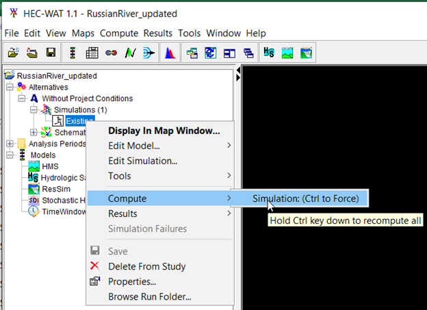
1. From the Study Tree, right-click the FRA simulation name, Existing and the shortcut menu opens. From the shortcut menu, point to Compute, and while holding down the Ctrl keyboard key, click Simulation (CTRL to Force) from the submenu.

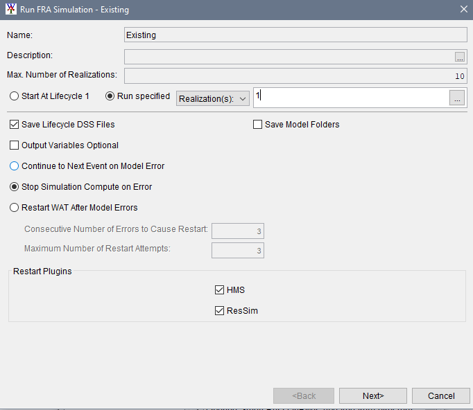
- This will bring up the Run FRA simulation – Existing editor. For our FRA simulation, we’ll choose to compute only the first realization, rather than the entire compute that is described in the FRA Simulation Editor.
2. From the top of the FRA Simulation Editor select the radio ![]() button for Run specified, and from the dropdown list, select Realization(s). In the textbox next to the Run specified dropdown list, enter "1" as the realization to compute.
button for Run specified, and from the dropdown list, select Realization(s). In the textbox next to the Run specified dropdown list, enter "1" as the realization to compute.

3. Click Next> and the compute information will display. Review the compute summary information, noting that under the title "Realization Information" the compute is set for "Lifecycles to Run:[1 – 10]" as these lifecycles form realization 1.
4. Click Compute and the Compute Progress window opens.
- In the Compute Progress window, you should notice only the Hydrologic Sampler’s portion of the compute, and then all events being skipped. This choice is to save time (with approximate compute time of around 43.2 seconds), to allow more realizations to be generated. Also, from the HEC-WAT main window, from the Messages Pane, notice that the following messages appear "INFO: Failed to delete … can not be deleted because it is not empty. Contains: [Existing.hsr, Existing.hsx]" which indicates that the filters were added successfully in Part 2 of this workshop.
5. Once the compute is complete, close the Compute Progress
Review the Results of the Modified FRA Simulation:
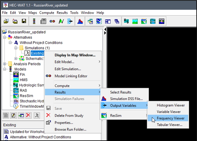
6. To view the results as a frequency curve, from the Study Tree, right-click on Existing FRA simulation, point to Results, point to Output Variables, and click Frequency Viewer from the shortcut submenu.

7. From the Variable list, select the RR_Precip-BASIN AVERAGE output variable produced by the Hydrologic Sampler. It might already be the selected variable. The figure below shows the viewer.

8. Close the Frequency Viewer window.
We would like to compare the results of sampling basin-average precipitation to the input precipitation frequency curve, to see if it matches. This is difficult to do from the Frequency Viewer, because the original frequency curve does not show. Therefore, we will move these results to the spreadsheet “workshop_inputs.xlsx” and plot them against the input curve.
9. Open HEC-DSSVue from the HEC-WAT main window, by clicking the HEC-DSSVue icon from the HEC-WAT toolbar (![]() ) icon from the HEC-WAT toolbar. HEC-DSSVue should open with the Existing simulation-level results DSS file.
) icon from the HEC-WAT toolbar. HEC-DSSVue should open with the Existing simulation-level results DSS file.

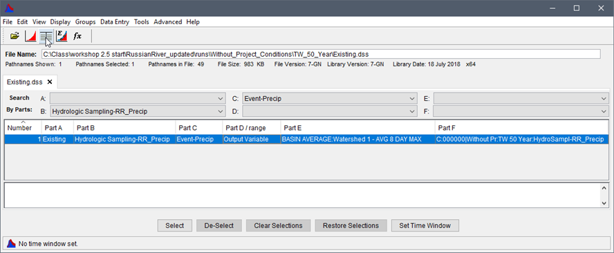
10. From the HEC-DSSVue window, from the File Name box, ensure that the path to the open DSS file is: "…\runs\Without_Project_Conditions\TW_50_Year\Existing.dss".
- From the DSS file locate the record for the RR_Precip, BASIN AVERAGE output. To find this record filter Part B to "Hydrologic Sampling-RR_Precip", filter Part C to "Event-Precip" and select the filtered record. Select the record with the pathnames shown below, which is the output variable record for the basin-average precipitation. It should be record number 20 in the file.

- Tabulate the record by clicking the Tabulate
 icon, from HEC-DSSVue toolbar. The tabulated record contains the precipitation (inches) for all ten lifecycles.
 - Copy the lifecycle precipitation data for the ten lifecycles by selecting only the cells in the 10 columns and 50 rows that hold precipitation values (ignore the first two columns and the first three rows), and clicking Ctrl+C.
11. Navigate to the open “workshop_inputs.xlsx” spreadsheet and select the “RZ1 Output” sheet. Select the upper-left corner of the blue cells (cell B3) and paste (Ctrl+V) the data.
- In the spreadsheet, select to the “GEV input and output” sheet to see the data plotted against the input 8-day precip frequency curve.

- Move to the “RZ1 GEV curve” sheet to see the data plotted against the new GEV curve sampled for this realization, with parameters found in the *.hsr file for realization 1.