WAT HMS Analysis

Last Modified: 2023-07-06 16:08:55.856

Software Version

HEC-WAT Version 1.1.0 was used to create this example. You can open the example WAT study with HEC-WAT Version 1.1.0 or a newer version.

Download Project File: StartModel.zip

Model Development: WAT workshop

This workshop uses data from Foster Joseph Sayers Dam located on Bald Eagle Creek in Centre County, Pennsylvania, about 70 miles northwest of Harrisburg, PA. There are two contributing tributaries located just downstream of the dam, Marsh Creek and Beech Creek. This workshop was made for the purpose of demonstrating HEC-WAT with HEC-HMS as the routing model. The Flood Risk Analysis (FRA) simulation mode (opposed to the event simulation mode) will be used in this workshop.

The purpose of this workshop is to show how you can sample from a flow frequency curve using the Hydrologic Sampler plugin with a simple reservoir built in HEC-HMS to produce a stage-frequency curve with uncertainty. The workshop provides a HEC-HMS project of Bald Eagle Creek and two excel files containing inputs to HEC-HMS and HEC-WAT.

The general workshop tasks are the following:

Start a new WAT project
Configure the Map Schematic and add the Common Computation Point
Import and configure the HMS model
Configure the WAT components
Set up the Hydrologic Sampler
Create a Simulation
Set up model Skip Rules
Select Model Output Variables
Set up Model Linking Editor
Compute Simulation
Review Results

Task 1: Start a New WAT Project

Open HEC-WAT and start a new study by selecting File | New Study. You will see the following dialogue box appear. Name your study Bald_Eagle_Creek. In the Directory field choose the WAT student workshop directory.
You must set a coordinate system upon starting any new project. Select the Edit button next to the empty Coordinate System field. Select Load from File and browse to the WAT student workshop directory. Select WAT_HMS | Common | Map Data | River_StatePlane.prj.

When applicable, always load the coordinate system from the existing HMS or ResSim model for consistency. The model files should contain the shapefiles with the applicable projection information
From this editor we can also add all the pertinent shapefiles needed for a WAT project with HMS. Select Add Map Layers. Use the explorer window to browse to the WAT student workshop directory. Select WAT_HMS | Common| Map Data then, holding the CTRL key select stream_align.shp, Reach.shp, and Subbasin.shp to add to the project.

Shapefiles can also be added in the primary WAT editor by selecting Maps | Add Map Layers at the top of the page then browsing to the correct folder. However, it is still recommended to load the stream alignment from the New Study editor. Adding the stream alignment first will assist the import of the other shapefiles.
Lastly, with the Create Default Alternative check box selected, select the Existing Conditions radial button as the Alternative Name. Press OK to create your project.

Task 2: Configure the Map Schmatic and add Common Computation Points

Verify that the correct plug-ins are available in the WAT. Go to Tools | Plugin Information. Verify that the HMSWATAdapter and the HydrologicSamplingPlugin are checked.
Convert the stream alignment shapefile into a WAT project stream alignment. The stream alignment shapefile was added when the study was created but it needs to be converted into a WAT stream alignment for the WAT to recognize it as the stream alignment. Navigate to Maps | Import | Stream Alignment. An import editor will appear as shown in Figure below.
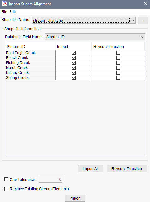
1. If Import All option is grayed out, click the “…” next to the Shapefile Name dropdown and navigate to HEC-WAT | Bald_Eagle_Creek | maps and select the stream_align.shp. All the streams are selected by default.
2. Select Import All at the bottom of the editor then close the editor. The map window should look something like the Figure below.
Select the Schematic tab at the bottom of the explorer window to view and manage map layers. The schematic should now show the shapefiles (Reach.shp, Subbasin.shp, and stream_align.shp) added to HEC-WAT when you started the new project.
Add a common computation point for the reservoir Bald Eagle Creek by clicking on the icon on the left side of the map schematic.
1. Holding the Ctrl button, add the point near the center of the basin and name the point Sayers Dam Inflow.
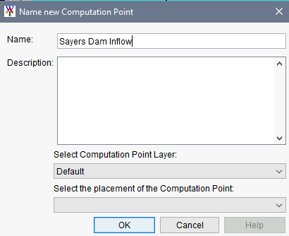
2. The exact location of the point is not important. Your map schematic should look like the figure below.

Task 3: Import and Configure the HMS Model

Ensure you are in the Study tab of the explorer window. Expand the Models option, you will see a number of icons appear. Right click on the HMS icon and select Import, then browse to the WAT_HMS | HMS Model | Bald_Eagle_Creek directory and select the Bald_Eagle_Creek.hms file to import. The HEC-HMS model will appear automatically and a message will appear stating that there is already an existing HEC-HMS model in the HEC-WAT project and is it ok to overwrite the existing model. Click the Yes button to overwrite an existing HEC-HMS model.
The HMS model will automatically open. Close HEC-HMS and HEC-WAT and open HEC-HMS software located in the apps folder of the HEC-WAT software package. Navigate to the Bald_Eagle_Creek.hms file and open the project in HEC-HMS.

While you can edit hms projects by launching hms through the WAT CAVI, working in the standalone HEC-HMS software is preferred. Fewer graphical issues have been reported by opening the project in the standalone version of hms.

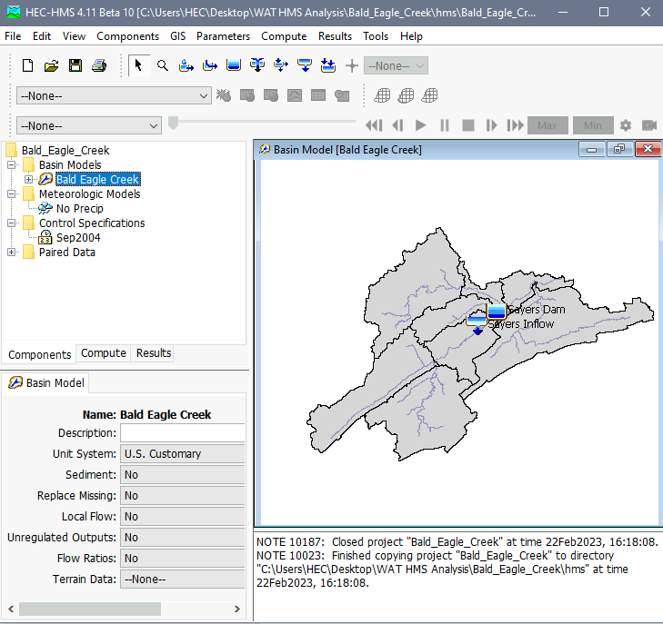
Note how the model is configured. The Basin model is named Bald Eagle Creek, Meteorological Model is named No Precip, and Control Specifications is named Sep2004. In the basin model, there is only a source element and a simple reservoir element. HEC-HMS does not perform downstream operations; however, ungated spillway flow conditions can be simulated.
First, we will need to import hydrograph shape sets. A copy of the June 1978, September 2004, and December 2010 inflow hydrographs have been added to the WAT project under the workshop directory ...\BaldEagleCreek\Common\Shapesets in a HEC-DSSVue file named Sayers_Inflow.dss. Using Windows Explorer, copy the Sayer_Inflow.dss file to the … \WAT_HMS\Bald_Eagle_Creek\hms\data folder.
In HMS, find the Components menu at the top of the screen, then select Components | Time-Series Data Manager. Once the Time-Series Data Manager Window opens, select Discharge Gages from the Data Type drop down menu, then select New. Change the name to Sayers Inflow and click Create. Close the Time-Sereies Data Manager Window.
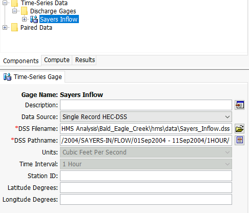
Click on the inflow gage you just created by expanding Time-Series Data| Discharge Gages in the project tree, then click on the Sayers Inflow gage, and you will see the input options in the component editor below.
Change the data source under the Time-Series Gage tab to Single Record HEC-DSS. Link the DSS file name by browsing to the \WAT_HMS\Bald_Eagle_Creek\hms\data folder. Double click on the Sayers_Inflow.dss file and set the Pathname to /2004/SAYERS-IN/FLOW/01Sep2004 - 11Sep2004/1HOUR/OBSERVED/ by clicking on the icon to the right of the DSS Pathname and selecting the record from the dialog box. When you are finished, the Time-Series Data should look like the figure below.
Connect the flow data you just entered to the Bald Eagle Creek basin model by expanding Bald Eagle Creek basin model in the project tree, clicking on the Sayers Inflow source element, clicking on the Inflow tab in the component editor, and selecting Sayers Inflow as the discharge gage. The Paired Data Elevation-Storage and Storage-Discharge Functions have been added for you. Before setting up an uncertainty analysis we will need to set up a simulation run for the data provided to make sure the model computes and reasonable results are generated
Go to the Compute menu and select Simulation Run Manager and create a new Simulation Run. Enter the name 2004 Event and follow the next button through the editor wizard. Select Bald Eagle Creek as the basin model. Select No Precip as the meteorological model. Select Sep2004 as the control specification and press Finish. Close the Simulation Run Manager dialog box.

We are only trying to feed the WAT the reservoir starting pool from HMS and therefore it is not necessary to have precipitation in your model. The meteorological model is still required, however, because HEC-HMS requires one to run.
From the Compute tab, expand Simulation Runs and click on the 2004 Event simulation. Click the compute button to begin the simulation. The simulation should only take a second. View results from the simulation at the source and reservoir elements, which can be found through the Results tab at the bottom of the window.
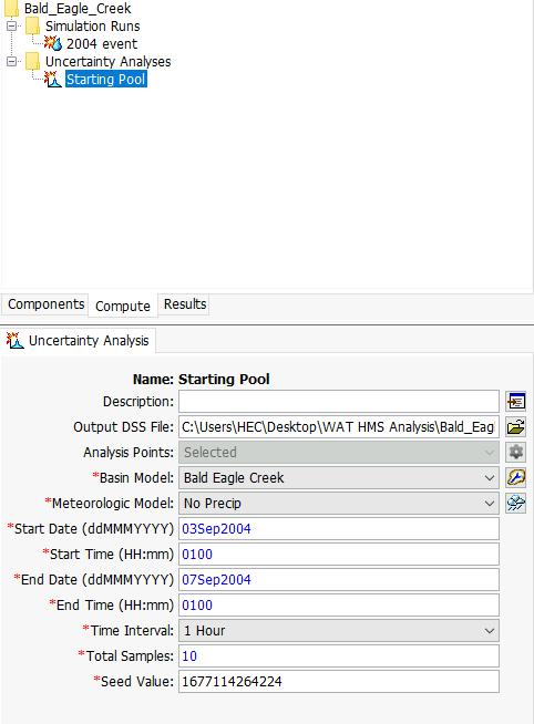
We will set up the Uncertainty Analysis. In order for the WAT to use Monte Carlo sampling of the reservoir starting pool, an uncertainty analysis must be set up in the HEC-HMS model. Navigate again to the Compute menu at the top of the screen and select Uncertainty Analysis Manager and create a new uncertainty compute. Enter the name Starting Pool then follow the next button through the editor wizard. Select Bald Eagle Creek as the basin model. Select No Precip as the meteorological model then push Finish. Close the Uncertainty Analysis Manager dialog box.
Select the uncertainty analysis you just created. In the uncertainty analysis Component Editor, enter the starting date 03Sep2004 01:00 and the ending date and time to 07Sep2004 01:00. Make sure the time interval is 1-Hour and change the Total Samples to 10, as shown in Figure below. This will inform HEC-HMS to run 10 simulations for the time window entered which will sample a new reservoir starting pool parameter for each of the simulations.
Right click on the Starting Pool uncertainty analysis and select Add Parameter.

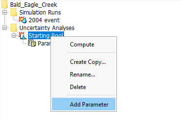
The parameter will appear as a menu option just below the Starting Pool title. Select it so that you see the component editor change.
Change the Element to Sayers Dam, the Parameter to Outflow Curve – Initial Elevation, the Method to Monthly Distribution, and the Distribution to Triangular. You will see the monthly distribution table change to reflect a triangular distribution of “Lower”, “Mode”, and “Upper”.
Navigate to the STATS_ReservoirStartingPool_v5.0_Sayers.xlsb workbook in the workshop folder ...\BaldEagleCreek\Common and open it. Find the Reservoir Starting Pool Stats tab in the workbook.
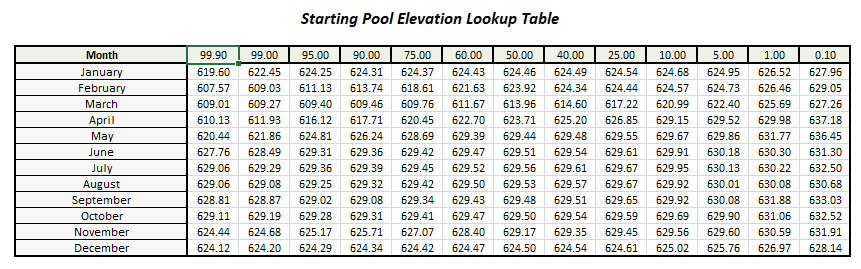
Copy the column for the 95 percent chance exceedance (95.00) from the "Starting Pool Elevation Lookup Table" and paste it into the “Lower” column of the table in HEC- Then copy the 50 percent chance exceedance (50.00) column from the reservoir starting pool stats tab and paste it into the “Mode” column of the table in HEC-HMS and finally, copy the 5 percent chance exceedance (5.00) column and paste it as the “Upper” column in the table in HEC-HMS. Type in 605 as the minimum value and 635 as the maximum value. When you are finished Parameter 1 should look like the Figure below.
Next we will select the HMS output that we want displayed. In the uncertainty analysis Component Editor, select the next to Analysis Points to open the Results editor. Select Select Pool Elevation as the output to save. Click Save and then Close.
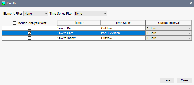
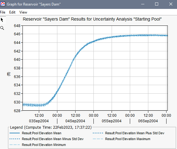
Now we will compute the Starting Pool Uncertainty Analysis in HEC-HMS. Right click on the Starting Pool uncertainty analysis and select Compute. The compute should only take a few seconds. View the results by navigating to the Results tab in the watershed explorer. Under the Uncertainty Analysis folder expand Starting Pool and select Pool Elevation. The resulting curve should look like the figure below.
Close the graph, click the Save, and then Close HEC-HMS.

Task 4: Configure the WAT Components

First we will set up the Program Order. In the WAT, the program order is used to set the sequence that individual programs are computed in the WAT simulation.

If all available plug-ins are active, the WAT will set up a default program order of HEC-HMS, HEC-RAS, HEC-ResSim, and HEC-FIA, respectively. We want to create a custom program order to reflect the fact that we are only using HEC-HMS in this project.

Select the Program Order icon in the ribbon at the top of the screen.
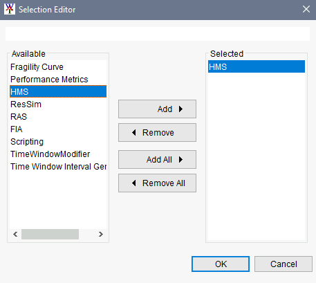
Select Program| New. Name the new order HMS then click Select Programs at the bottom of the dialogue box. The selection editor will appear. Select HMS and click Add as shown in the figure below, then press OK and close all three dialog boxes.
Set up the Analysis Period. For ease of outputting data and visualizing results, the WAT will split the Flood Risk Analysis (FRA) simulations, which are comprised of realizations and number of years per realization, into smaller groups known as Lifecycles. The WAT divides the number of years in a realization by the length of the analysis period to determine the number of lifecycles per realization. Thus, an analysis period of 500-years would result in 20 lifecycles in a simulation with 10,000 years per realization. Since this analysis is not for computing damages over typical lifecycles (30 and 50 years) the length of the analysis period is arbitrary. Either select analysis periods that are 100 or 500 years long when performing a loading curve analysis.
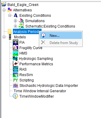
1. In the Study tab of HEC-WAT’s project tree, right click on Analysis Periods in the explorer window and select New.
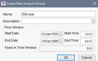
2. Name your analysis period 500-year and then fill in the time window from 01Jan1500 0000 to 31Dec1999 2400. Even though the time period can be an arbitrary selection of dates, the analysis period must include a full 500 years. Double check that it reads 500 in the Years in Time Window display as shown in Figure and click OK.

Task 5: Set Up the Hydrologic Sampler

The Hydrologic Sampler provides the WAT FRA compute sequence with the data input required for sampling flow or precipitation.

Expand the menu next to the Models folder in the study tree. Right click on the icon for Hydrologic Sampling , and select New. The dialogue box to create a new Hydrologic Sampling Alternative should appear. Name the alternative Flow Sampler and press OK when you have finished. The following screen shown below should open.
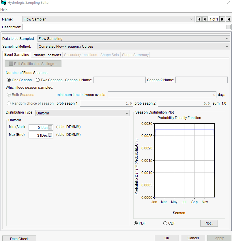
In the Event Sampling tab, change the Distribution Type to Empirical (graphical). The table that appears in the editor is where you will enter your flood seasonality statistic
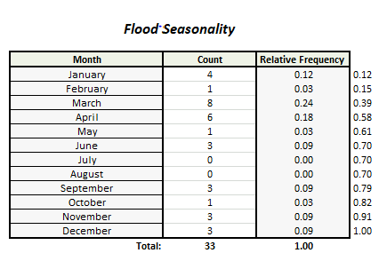
Navigate to the STATS_FloodSeasonality_v5.0_Sayer workbook in the workshop folder ...\BaldEagleCreek\Common and open it. Find the Flood Seasonality Stats tab in the workbook. Use the values next to the Relative Frequency column in the Flood Seasonality table. This is the calculated cumulative probability. Copy and paste these calculated cumulative probability values into Cumulative Probability column in the empirical data table in the WAT. The very first row much have a value of 0 and the last row must have a value of 1.0. Manually edit the dates in the Date column, the first row is January 1, and then the remaining rows are the last day of the following month. Click Apply once you have entered all the information shown as shown in the figure below.

The relative frequencies found in the flood seasonality editor must be converted to a cumulative probability distribution. Accumulate your frequencies and add them to the table chronologically. Notice also that values cannot be repeated so you may need to manually adjust values otherwise you will receive an error during simulation
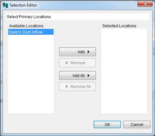
Navigate to the Primary Locations tab within the editor. This tab allows you to link your event hydrograph(s) to your primary inflow location(s). Click on the Select Primary Locations. A dialogue box will appear that will allow you to select as many headwater locations as desired. We only have one reservoir in this example. Select Sayers Dam Inflow, click Add, then and press OK.
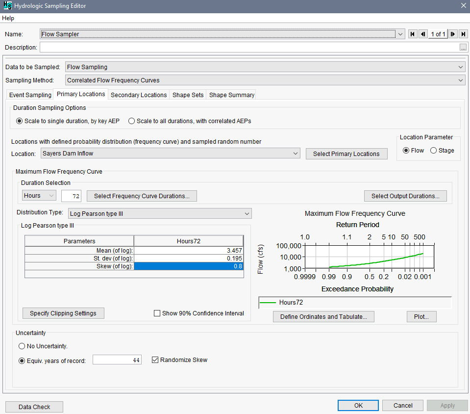
Under Duration Sampling Option change the Duration of Maximum Average Flow to 72 Hours. Change the Distribution Type to Log Pearson type III. Fill in the rest of the Volume-Duration-Frequency statistics. These statistics are from a Bulletin 17C analysis at a stream gage with 44 years of record. Enter Mean of 3.457, Standard Deviation of 0.195, Skew of 0.8, and Equivalent Years of Record of 44. Click the check box to turn on Randomize Skew. When you are finished, the editor should look like the figure below.
Navigate to the Secondary Locations This is where you can add additional inflow locations such as tributaries. Since HEC-HMS does not perform downstream operations we do not need to include any downstream inflows.
Navigate to Shape Sets. In this tab you will link your event inflow hydrographs to the hydrologic sampler. As previously mentioned, we have identified three hydrographs for this model from the December 2010, September 2004, and June 1978 events. The event hydrographs have been saved to a DSS file Sayers_Inflow.dss in the ...\BaldEagleCreek\Common\Shapesets folder. Copy the Sayers_Inflow.dss file from the Common directory into shared folder in the HEC-WAT project ...\Bald_Eagle_Creek\shared. Now, click on New Set and label the hydrograph December 2010.

When you are working in the WAT it is a good idea to save the shape sets you wish to use separate from the rest of the period of record and in the shared folder of your model directory.
With the Sayers Dam Inflow full pathname highlighted in the lower table, press “Select DSS Path”, click on the folder browser, and browse to the model directory Shared folder. Select the Sayers_Inflow.dss file and navigate to the December 2010 hydrograph. Select pathname. Close the DSS selector window. Your Hydrologic Sampling Editor should now look like the figure below.
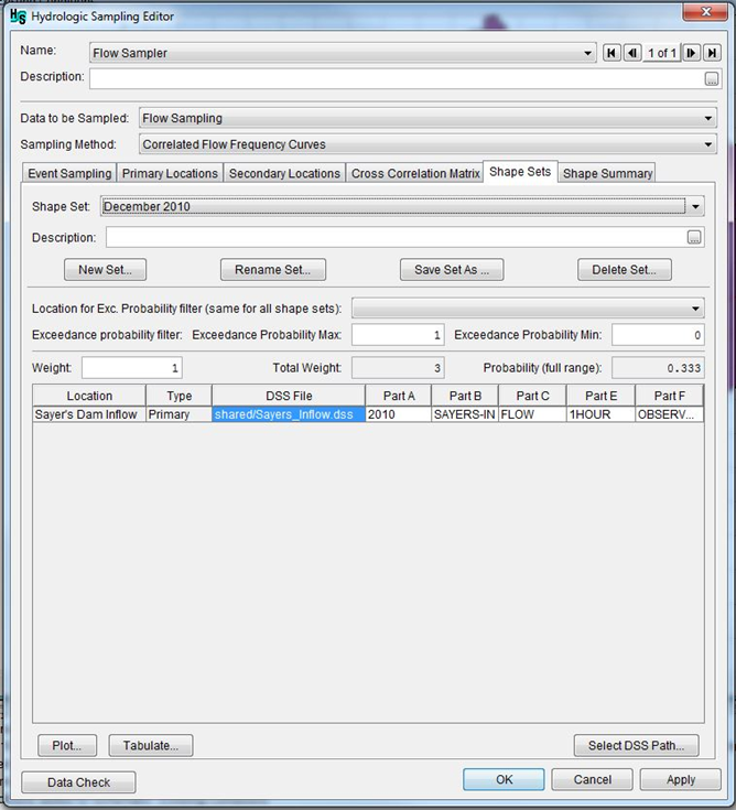
When you have finished linking the first set, select New Set and repeat the process for both the September 2004 and June 1978. Make sure the Location for Exc. Probability Filters is set to Sayers Dam Inflow. You only need to do this once for the selection to apply to all the hydrograph shape sets.
Navigate over to the Shape Summary tab. Leave all hydrograph weights equal to 1. When you are finished adding shape sets press OK on the editor to return to the main screen. You are finished with the Hydrologic Sampler.
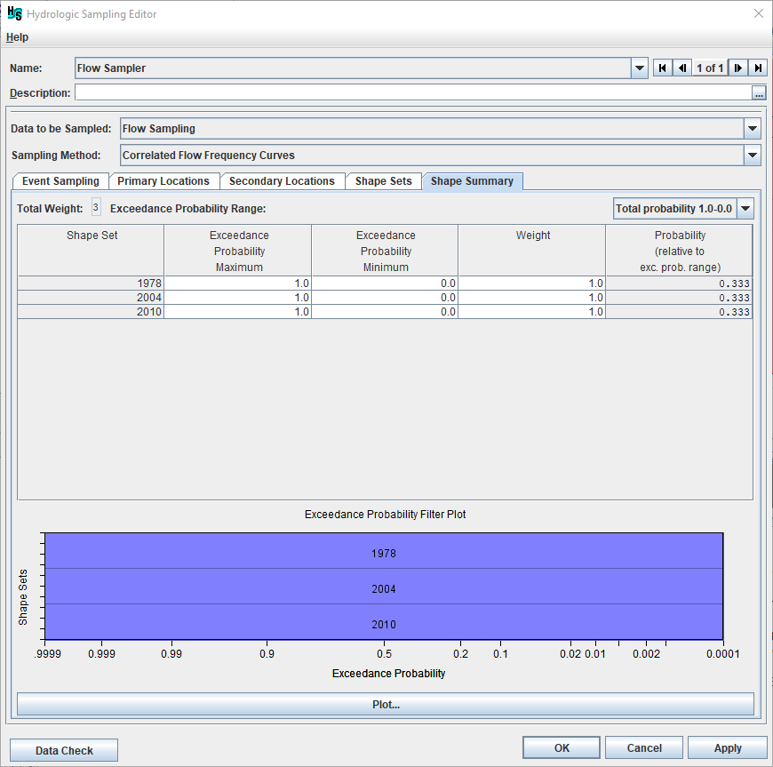
The WAT will automatically set the probability of sampling of each hydrograph based on the weight assigned to each hydrograph. The default value is 1. If you would like to assign a different sampling probability to your events then you must manually change their weights. You can see a graphical representation of the weights on the Shape Summary tab.

Task 6: Create Simulations

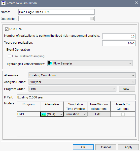
Expand Alternatives and Existing Conditions on the study tree. Right click on the Simulations folder and select New. The Create New Simulation dialogue box will appear. Name your project Bald Eagle Creek FRA. Check the box Run FRA. By checking FRA (Flood Risk Analysis) you turn on Monte Carlo sampling.
You will see a new set of options appear under the FRA check box. Here we will enter the number of realizations and years you want to run per realization. Within the WAT/FRA compute, the user must select the number of years per realization and the number of realizations per simulation. For example, the user can choose 10,000 years per realization and then 100 realizations. In this example, 10 separate realizations of 1,000 years will be simulated, providing 10 flow and stage frequency curves that extend to 1/1,000 ACE (by sorting and ranking the flows/stages then dividing the rank by the total number of years in a realization, 1,000). Ten realizations do not provide enough information to define the uncertainty around the expected probability curve. However, in order to reduce computation time, for the purposes of this workshop we will reduce the number of realizations and events. Enter 10 for the number of realizations and 1,000 for the years (events) per realization.

In general, the number of events per realization should be two to three times the frequency storm event desired. For example, if the 1/100 pool elevation is desired, sampled events for each realization should be a minimum of 250.
Next, use the drop down box under the “Hydrologic Event Alternative” label to select Flow Sampler as the Hydrologic Event Alternative. Make sure the Alternative is set to Existing Conditions. Use the Analysis Period drop down box to select the 500-year. Use the Program Order drop down box to select the HMS uncertainty analysis. In the Models section, use the drop down box to select (MCA)Starting Pool as the HMS Alternative. When you are finished, the simulation editor should look like the figure below.
Select OK to return to the main screen. You should see the simulation you just created appear under the Simulation folder in the study tree.

Task 7: Model Skip Rules

Model skip rules allow the user to skip low flow events during simulation that are lower than a predetermined threshold. This is done to reduce compute time only.

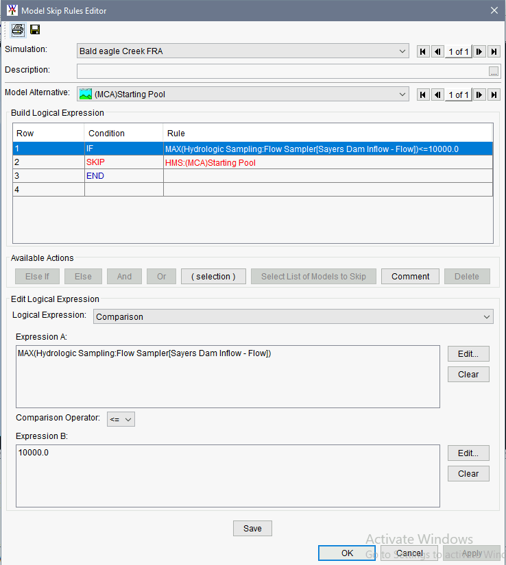
Click on the Model Skip Rules Editor icon in the ribbon at the top of the page. You will see the Skip Rules Editor appear. Select Bald Eagle Creek FRA as the simulation and (MCA)Starting Pool as the Model Alternative.
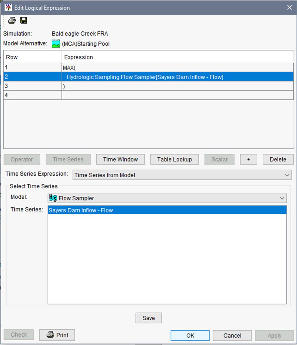
Select the IF line to highlight and select the Edit button next to the Expression A box. An additional dialogue box entitled Edit Logical Expression should appear.
Ensure that the first row of the Logical Expression editor is highlighted. Select Operator. Select MAX as the operator from the drop down menu. Move to the second row in the editor. Select Time Series. Change the Time Series Expression to Time Series from Model using the drop down box next to the label. Using the drop down box next to the Model label, select Flow Sampler as the hydrologic sampling model. The editor should look like the Figure below. Next, select Sayers Dam Inflow as the time series. Hit Apply. When you are finished, press Save and then OK to return to the main Model Skip Rules editor.
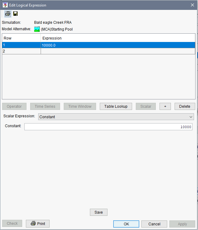
With the IF line still highlighted, select the Edit button next to the Expression B box. An additional dialogue box titled Edit Logical Expression should appear. Make sure that the Scalar option is chosen, and that the Scalar Expression is set to Constant. Then, enter 10,000 for the constant value. The editor should look like the Figure below. Hit Apply. When you are finished, press Save and then OK to return to the main Model Skip Rules editor.
Now, highlight the second row in the main editor which is currently titled END. Once it is highlighted, click on Select List of Models to Skip. The END title will change to SKIP and a rule will now need to be set. Under the Select Models to Skip title, check the box next to the HMS alternative (MCA)Starting Pool as the skipped model. Hit Apply
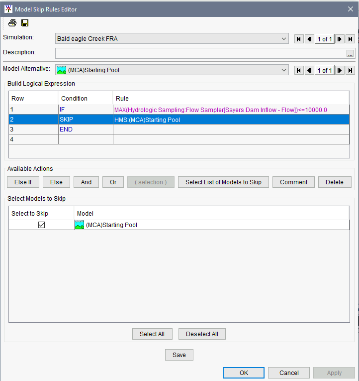
Select Row 1 to return to the main editor. The final expression should look like the figure below. Press Save and then OK when you have finished to close the Skip Rules Editor.

Task 8: Select Model Output Variables

The WAT FRA simulation produces hundreds of outputs. In order to streamline your results, the model output editor allows you to specify what output you want the program to write to a DSS file.

Select the Output Variable Editor from the ribbon at the top of the screen. Using the drop down menu to select the simulation that you created entitled Bald Eagle Creek FRA.

You will need to add the desired output from the Hydrologic Sampler and HMS model separately.
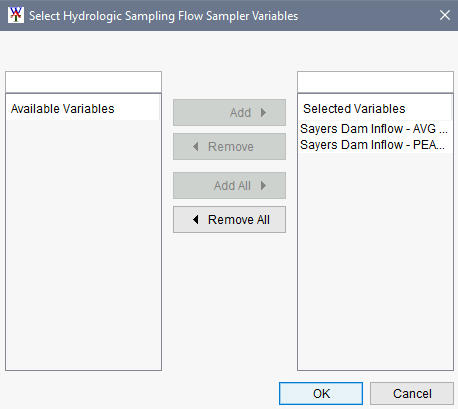
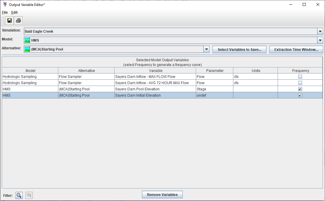
First, using the drop down menu select Hydrologic Sampling as the Model. Using the drop down menu and select Flow Sampler as the Alternative. Click on Select Variables to Save. An additional dialogue box will appear. Double Click on the variables Sayers Dam Inflow-AVG 72 HOUR MAX Flow and Sayers Dam Inflow-MAX Flow. Press OK when finished.
Next, change the Model to HMS and the Alternative to (MCA)Starting Pool. Click on Select Variables to Save. From the dialogue box that appears select the variables Sayers Dam Pool Elevation and Sayers Dam Initial Elevation. Press OK to return to the Output Variable Editor page.
When you have finished adding the variables, the editor should look like the Figure below. Select the Frequency check box next to the HMS output Sayers Dam Initial Elevation and Sayers Dam Pool Elevation so that the program will compute the frequency curve for these outputs. Save and then close the box.

Task 9: Set up the Model Linking Editor

As the name suggests, the Model Linking Editor defines how model output is linked from the models in the WAT compute sequence.

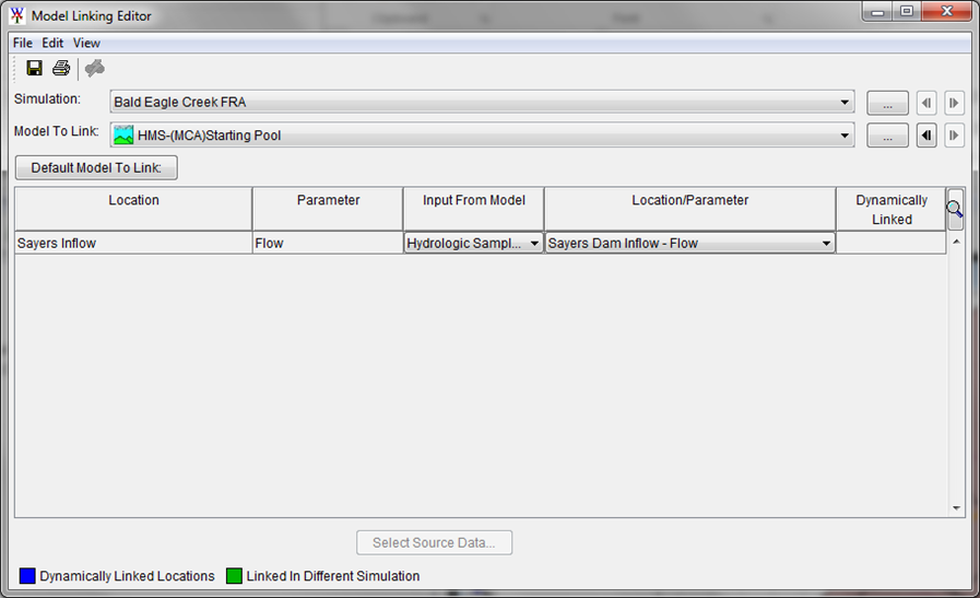
Select the Model Linking Editor from the ribbon at the top of the screen . Select Bald Eagle Creek FRA as the Simulation and HMS-(MCA)Starting Pool as the Model to Link. You will see additional information appear at the bottom of the editor.
Under the Input from Model column, change the drop down menu to read Hydrologic Sampling-Flow Sampler. Make sure the Location/Parameter option is correctly set to Sayers Dam Inflow - Flow. Save and close the editor.

Task 10: Compute a Simulation

You are now ready to compute a simulation.

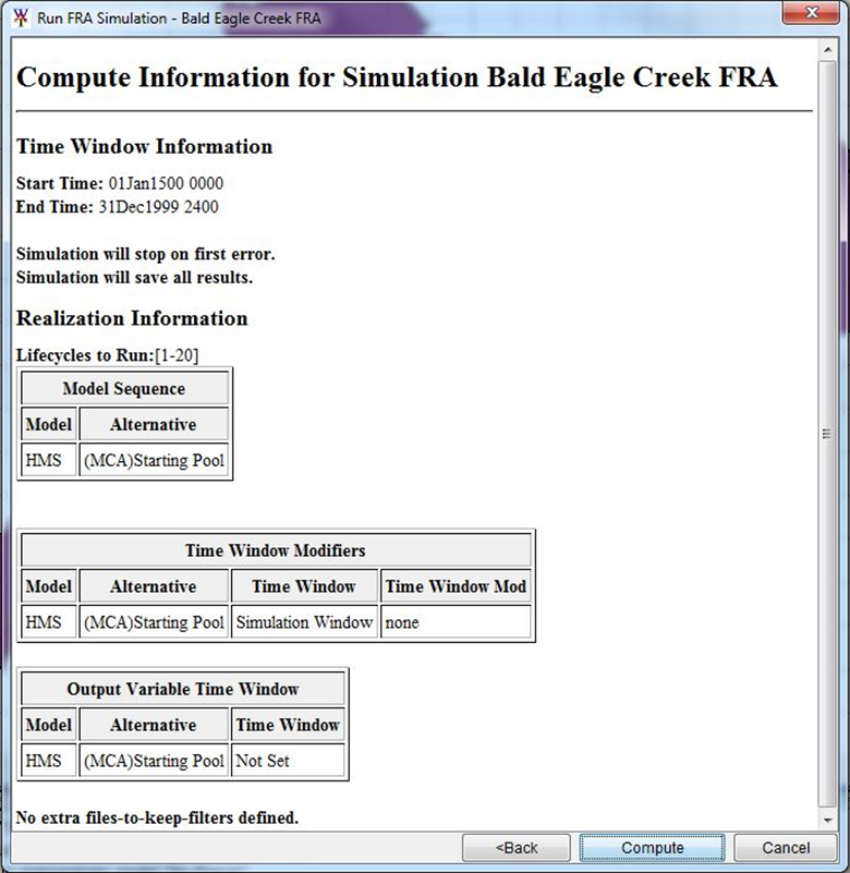
Expand the Simulations folder in the study tree (in the Existing Conditions alternative). You should see the simulation you created (Bald Eagle Creek FRA) appear. Right click on the simulation and select Compute| Simulation. A dialogue box should open labeled Run FRA Simulation-Bald Eagle Creek FRA.
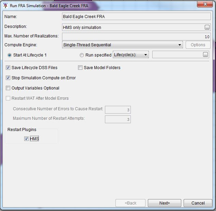
Make sure the box is checked to restart the HMS Plugin at the end of each lifecycle. Select Next to review the simulation summary sheet and review all the model parameters. Select Compute. The compute should take about 10 minutes.

Task 11: Review Results

The results can be easily viewed by selecting Results| Output Variables| Frequency Viewer from the HEC-WAT menu bar. Select the Sayers Dam Pool Elevation option from the Variable drop down list. Select All Realizations from the Realization drop down list. The plot should update showing peak reservoir stage for all 10 realizations, the combined (expected probability) stage frequency curve, and then the 5 and 95 percent confidence limits. See the figure for the stage-frequency curve. Notice that the low end of the curve is truncated due to large skip flag defined to reduce the compute time for this workshop.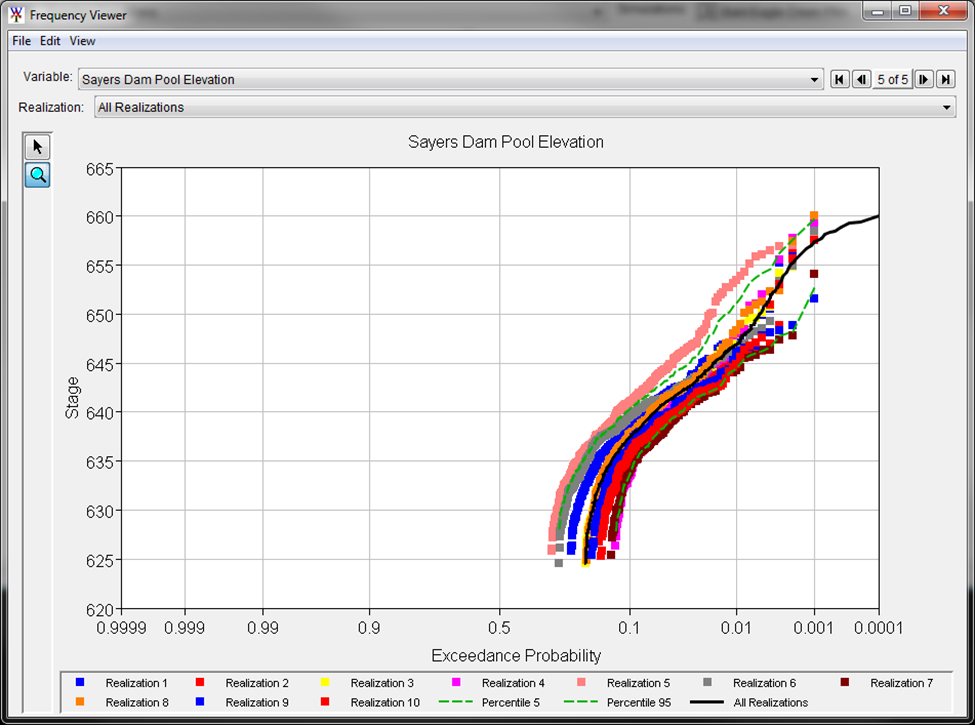

Conclusion

That's it! Download and review the solution project compare with yours to see how you did!

Download Final Project File

FinalProject.zip

Return to top of page.