Reservoir Inflow

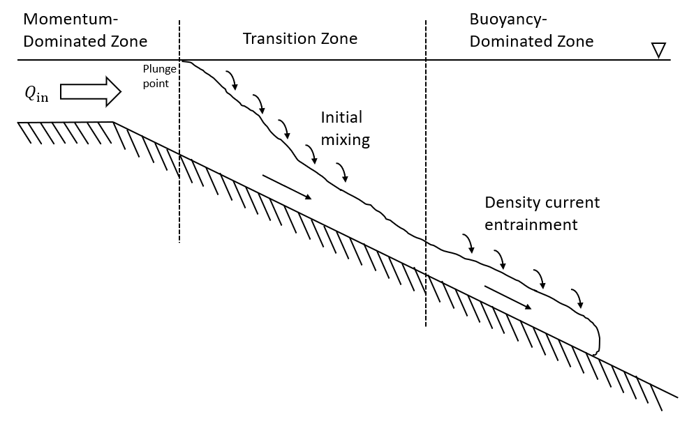
When water from an inflow enters a reservoir, it typically passes through three zones. Near the entrance to the reservoir, the inflow is dominated by the momentum of the inflowing water. After a transition zone where there is some initial mixing, the movement of the inflow current becomes dominated by the difference in density between the inflowing water and the upper layers of the reservoir. Warmer, less dense inflows spread out along the surface of the reservoir and are called overflows. Colder, denser inflows plunge and run along the bottom of the reservoir, drawing in water from the reservoir as they flow. If the inflow plunges to reach reservoir layers of equal density, the flow is inserted at that elevation in the reservoir as an interflow. If the inflow is cold enough to plunge to the bottom of the reservoir, it is known as a underflow. The figure below (redrawn from Fleenor, 2001) shows a plunging inflow.

Schematic showing three zones of mixing for a plunging inflow. The first zone is where momentum from the river dominates. The second zone is a transition zone. The third zone is where the buoyancy of the entrained inflow is the largest factor contributing to inflow behavior.

Overflows

If the density of the inflow is less than the density of the top reservoir layer, the inflow enters the reservoir at the surface. The thickness of the overflow can be calculated following Yih (1958) as

1)	$\begin{array}{l}\displaystyle h_s = 1.35\left(\frac{q_\textrm{in}^2}{g\frac{\Delta\rho}{\rho_\textrm{in}}}}\right)^{1/3}\end{array}$

where

$\begin{array}{l}h_s\end{array}$ is the thickness of the overflow [m],
$\begin{array}{l}q_\textrm{in}\end{array}$ is the inflow rate per unit width [m²/s],
$\begin{array}{l}g\end{array}$ is acceleration due to gravity [m/s²],
$\begin{array}{l}\Delta \rho\end{array}$ is the density difference between the inflow layer and the reservoir surface layers [kg/m³], and
$\begin{array}{l}\rho_\textrm{in}\end{array}$ is density of the inflow [kg/m³].

Before the overflow is allocated to the reservoir layer inflows, a determination of the depth of the surface mixed layer is made. This is done by starting at the surface layer and proceeding to deeper layers while checking the density gradient. The discrete density gradient is defined below, and the limit of the surface mixed layer is defined when the gradient exceeds a user-defined tolerance, $\begin{array}{l}\epsilon\end{array}$ (default value 0.01 kg/m²).

$\begin{array}{l}\displaystyle \frac{d\rho}{dz} \approx \frac{\rho_{i-1}-\rho_i}{z_i-z_{i-1}} > \epsilon\end{array}$

where

$\begin{array}{l}\rho_i\end{array}$ is the density of $\begin{array}{l}i^{\textrm{th}}\end{array}$ the reservoir layer [kg/m³], and
$\begin{array}{l}z_i\end{array}$ is the center elevation of $\begin{array}{l}i^{\textrm{th}}\end{array}$ the reservoir layer [m].

If the overflow is contained within the surface mixed layer, it is distributed throughout the entire depth of the surface mixed layer uniformly based on layer volume. If the thickness of the overflow exceeds the depth of the mixed layer, normalized layer velocities and flows are calculated using the parabolic velocity determination used in the outlet flow calculations.

Plunging Flows and Entrainment

When negatively buoyant inflows enter a reservoir, they flow along the reservoir bottom (often a submerged river valley) until they reach the reservoir level with matching density. As these flows pass through the upper layers of the reservoir, they entrain some fraction of the warmer water, increasing the magnitude of the inflow intrusion and decreasing the density. This acts to transport some heat from shallower layers of the reservoir to deeper layers. Inflow density and in-reservoir entrainment determine the density of the inflow intrusion and thus the elevation where flows enter the reservoir. This physical process is modeled explicitly in 2D models (e.g., CE-QUAL-W2) but needs to be parameterized in 1D reservoir models.

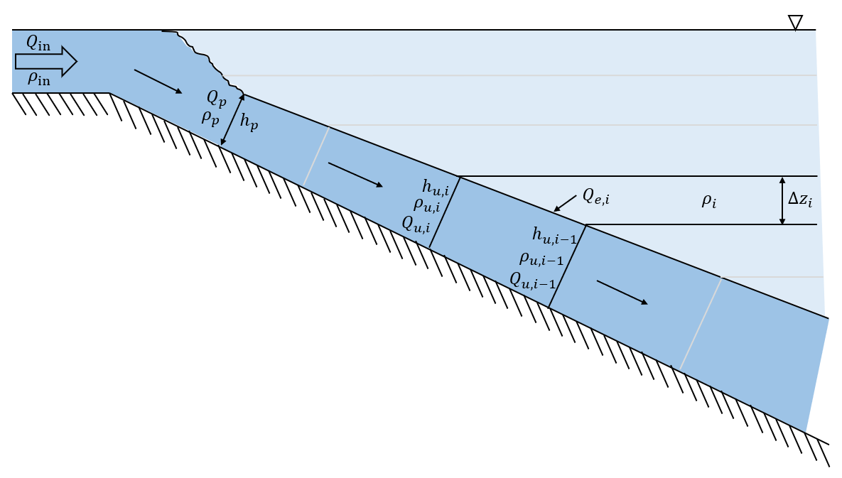
When the inflow first enters the reservoir, there is an initial mixing associated with the plunge location

$\begin{array}{l}\displaystyle Q_p = Q_{\textrm{in}} (1 + \delta)\end{array}$

where

$\begin{array}{l}\delta\end{array}$ is the initial mixing ratio [unitless],
$\begin{array}{l}Q_p\end{array}$ is inflow magnitude at the plunge point [m³/s], and
$\begin{array}{l}Q_{\textrm{in}}\end{array}$ is the original river inflow [m³/s].

For river inflows with mild slopes (less than 0.007), $\begin{array}{l}\delta\end{array}$ was found to be around 0.15 (Akimyama & Stefan, 1987). However, this parameter can vary significantly, and is user-defined for each major reservoir inflow in HEC-ResSim.

The depth at the plunge point is calculated following the analysis of Hebbert et al. (1979) for a channel with a triangular cross-section:

$\begin{array}{l}\displaystyle h_p = \left[\frac{2Q_p^2}{\left(F_p^2 \frac{g\Delta\rho}{\rho_\textrm{in}} \textrm{tan}^2(\phi) \right)}}\right]^{1/5}\end{array}$

where

$\begin{array}{l}h_p\end{array}$ is plunge point depth [m],
$\begin{array}{l}\phi\end{array}$ is the half angle of the river cross-section [radians], and
$\begin{array}{l}F_p\end{array}$ is the Froude number for the river at the plunge point [unitless].

The Froude number is defined by Hebbert et al. (1979) as:

2)	$\begin{array}{l}\displaystyle F_p^2 = \frac{\textrm{sin}(\phi)\, \textrm{tan}(S_o)}{C_D} \left(1 – 0.85 \, \sqrt{C_D} \, \textrm{sin}(\phi)\right)\end{array}$

where

$\begin{array}{l}S_o\end{array}$ is the slope of the submerged river channel [unitless], and
$\begin{array}{l}C_D\end{array}$ is the drag coefficient (unitless and assumed to equal 0.04).

In HEC-ResSim, the slope can be calculated based on provided reservoir elevations, or it can be user-defined. The river cross-section half angle is user-defined (default value 85°).

Once the depth and flow at the plunge point are determined, a series of successive calculations is performed starting at the top layer of the reservoir and proceeding deeper. At the start of each layer $\begin{array}{l}i\end{array}$ , the density of the underflow ( $\begin{array}{l}\rho_{u,i}\end{array}$ ) is checked against the density of the layer ( $\begin{array}{l}\rho_i\end{array}$ ). If the underflow is denser than the layer, the depth of the underflow ( $\begin{array}{l}h_u\end{array}$ ) is updated according to Imberger and Patterson (1981):

$\begin{array}{l}\displaystyle h_{u,i-1} = \frac{6E}{5} \frac{S_o}{\Delta z_i} + h_{u,i}\end{array}$

where

$\begin{array}{l}E\end{array}$ is the entrainment rate [unitless],
$\begin{array}{l}\Delta z_i\end{array}$ is the layer thickness [m], and
$\begin{array}{l}S_o / \Delta z_i\end{array}$ is the longitudinal distance traveled by the underflow [m].

Then the increase in flow is calculated:

$\begin{array}{l}\displaystyle Q_{u,i-1} = Q_{u,i} \left(\frac{h_{u,i-1}}{h_{u,i}} \right)^{\frac{5}{3}}\end{array}$

and the underflow density updated:

$\begin{array}{l}\displaystyle \rho_{u,i-1} = \rho_{u,i} \left(\frac{h_{u,i-1}}{h_{u,i}} \right)^{\frac{5}{3}}\end{array}$

The procedure continues until the density of the inflow is less than the reservoir layer density, or the inflow reaches the bottom layer.

Schematic of the definitions for variables used in entrainment calculations. The depth (h), density (rho), and flow (Q) of the inflow are updated as it passes through each vertical layer of the reservoir. The inflow passes through the layers obliquely as it runs down the side slope of the reservoir.

Once the vertical location of the inflow is determined, the thickness of the inflow is calculated using Equation 1).

Entrainment Coefficient

The entrainment coefficient, $\begin{array}{l}E\end{array}$ , can be estimated by (Imberger and Patterson, 1981):

3)	$\begin{array}{l}\displaystyle E=0.5\,C_k\,C_D^{3/2}\,F_p^2\end{array}$

where

$\begin{array}{l}C_k\end{array}$ is an experimental constant (unitless and assumed equal to 3.2),
$\begin{array}{l}C_D\end{array}$ is the drag coefficient (unitless and assumed equal to 0.04), and
$\begin{array}{l}F_p\end{array}$ is the Froude number at the plunge point (Equation 2).

A consequence of this formulation is that the entrainment rate is constant throughout the simulation. In HEC-ResSim, it can either be calculated according to Equation 3), or entered as user input.

Inflows Entering at Depth

Inflows may be prescribed to enter the reservoir below the surface. This may be done for storm sewer outfall pipes which enter the reservoir at depth, or to account for the effect of a thermal curtain near the area of the inflow.

Similar to the logic for an inflow entering the surface, the density of the inflow is compared to the density of the reservoir water (at the depth of the inflow). Denser inflows are assumed to act like plunging inflows, and the calculation procedure described above is applied starting at the inflow depth, instead of the surface. Inflows that are less dense than the reservoir layer are assumed to mix upward, as necessary, until a stable density profile is obtained.