Task 2: Calibrate Inflow to Lake Mendocino and Lake Sonoma

In this task, we are going to use the HEC-HMS Combined Parameter Editor to calibrate modeled inflow to both reservoirs. 

1. Select the HEC-HMS node in the Forecasts window, then click the Combined Parameter Editor action button as shown below.
   
2. Open HEC-HMS results at the Calpella Gage junction and Coyote reservoir elements. Notice in the figure below, plots are open as well as summary tables. Using the correct output options can help you to quickly identify model performance and help guide you when making model adjustments. Notice how poor the model performs in the lookback period. Poor performance in the lookback period provides little confidence in the forecast period. 
   
   At the bottom of the Combined Parameter Editor is a drop down that lets you choose computation points in the model. Choose the Coyote computation point. When you press the compute forecast button on the bottom left of the Combined Parameter Editor, HEC-HMS will only run the model to the selected location. You should notice the simulation runtime is less when only computing the model to computation points.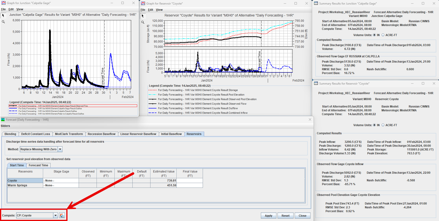 
   
   
   
   

   Modeling the correct amount of runoff volume is critical for reservoir elements. The Percent Bias metric is helpful for identifying how well the model performs when predicting runoff volume. A negative percent bias means the model is underpredicting runoff volume and a positive percent bias means the model is overpredicting runoff volume. Your goal is to have a percent bias close to 0 percent. 

3. Go to the Reservoirs tab within the Combined Parameter Editor. The Reservoir editor has a couple of time-saving options. 
   1. Make sure the Replace All With Zero option is selected for the discharge time-series data handling option (this option is important for those reservoirs configured to use an observed flow gage for the reservoir discharge). HEC-HMS will replace reservoir releases with 0 cfs for the forecast period (observed releases are used for the lookback period). HEC-HMS includes a simple rule-based operations option that could be useful when forecasting reservoir releases. 
      
      Next, select the Coyote Elevation stage gage for the Coyote reservoir and the Warm Springs stage gage for the Warm Springs reservoir. Notice HEC-HMS automatically extracts the elevation at the beginning time of the simulation. You no longer have to manually enter the reservoir elevation every time you create a new forecast, this option will automatically set the correct beginning elevation for you.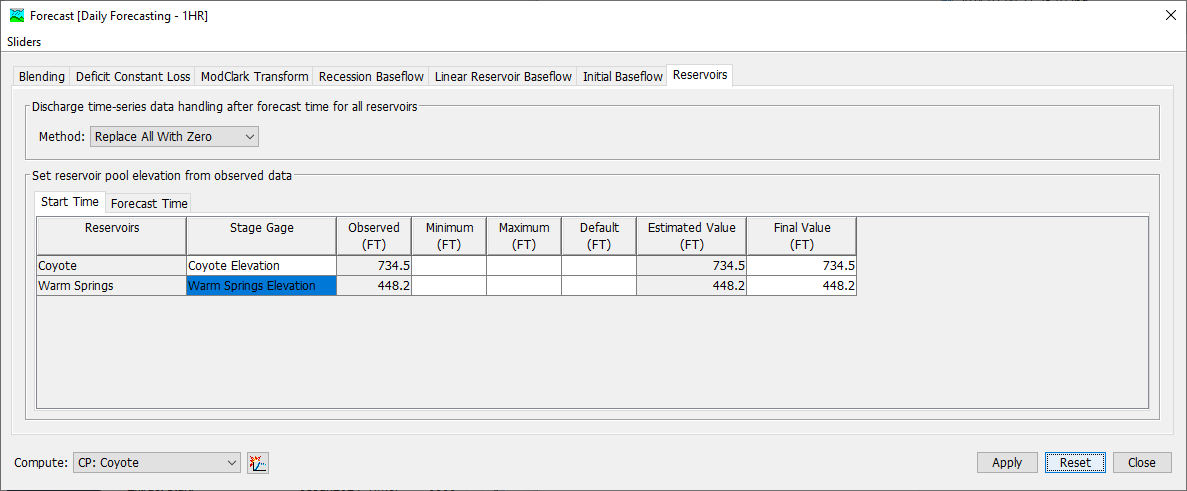 
      
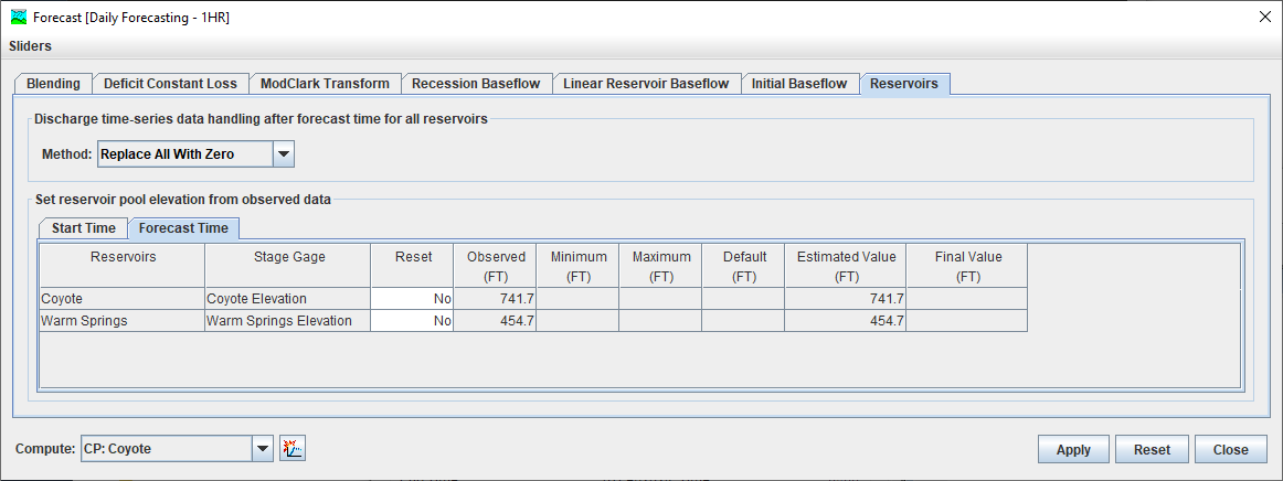
   2. The Forecast Time tab has an option to automatically Reset the reservoir elevation at the time of forecast. HEC-HMS will automatically adjust the simulated reservoir elevation to the observed elevation at the simulations forecast time. For now, leave this option set to No. 
      
4. Press the HEC-HMS compute bottom of the Combined Parameter Editor. As shown below, the starting reservoir elevation (on Jan 5th) now matches the observed data. There is still work to be done to improved the computed inflow into the reservoir. 
   
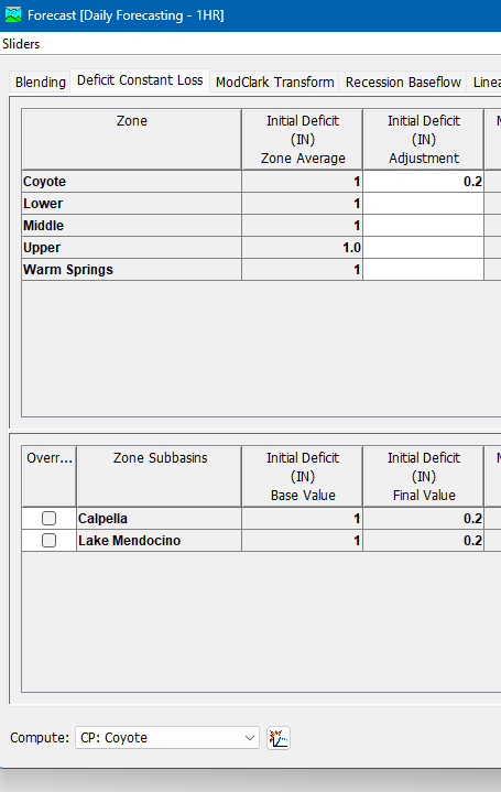
5. Open the Deficit Constant Loss tab in the Combined Parameter Editor. Notice the Coyote zone has two subbasins, Calpella and Lake Mendocino. The upper table is referred to as the zonal override table and the lower table is referred to the element override table. The upper table allows you to quickly edit parameter values for all subbasins in the zone. The lower table allows you to make parameter edits to individual subbasins. 
   
6. Enter a Zonal Override of 0.2 inches for the Initial Deficit for the Coyote Zone. The simulation time window started when the watershed was fairly wet. Click the Apply button and notice the zonal value is populated in the element override table (shown below).
   
7. Click the Compute button. You will not notice much difference in the computed flow hydrograph, the computed reservoir stage hydrograph does improve because higher runoff volume is computed (we decreased initial losses). 
8. The next step is to adjust the constant loss rate. You can use a multiplier in the zone override table. Enter *0.5 for the Constant Rate for the Coyote zone. Click the Apply button. The original constant loss rate values were multiplied by 0.5, as shown below. 
   
9. Rerun the simulation. As shown below, the computed flow at the Calpella Gage is much improved. The Nash-Sutcliff has improved to 0.733 (Percent Bias at 30.86 percent). The simulated reservoir elevation is much improved too. 
   
10. Before making additional adjustments to the constant loss rate, evaluate the baseflow/interflow response. The Linear Reservoir baseflow method is used for the subbasins in the Coyote zone. This baseflow method works nicely with the Deficit and Constant loss method. Precipitation that infiltrates once the soil moisture deficit has reached 0 inches is "routed" to the linear reservoir baseflow model. The GW 1 and GW 2 Fraction parameters are used to partition infiltrated water (when the soil is saturated) to each groundwater layer (fraction values do not need to sum 1, but the sum cannot be larger than 1). The model has been configured so that GW 1 simulates the faster responding interflow and GW 2 simulates the slower responding baseflow. More than likely, the only linear reservoir parameters you will need to adjust when calibrating a model in real-time are the fraction parameters. The other linear reservoir parameters should be consistent between events and not need adjustment. You should see a natural response with the fraction parameters. Seasonally, the GW 1 and GW 2 fractions should be larger in the winter as groundwater tables rise because vegetation is transpiring less. 
    
    Notice the observed and simulated results below. The results in the red circles indicate too much volume in the baseflow between the peaks.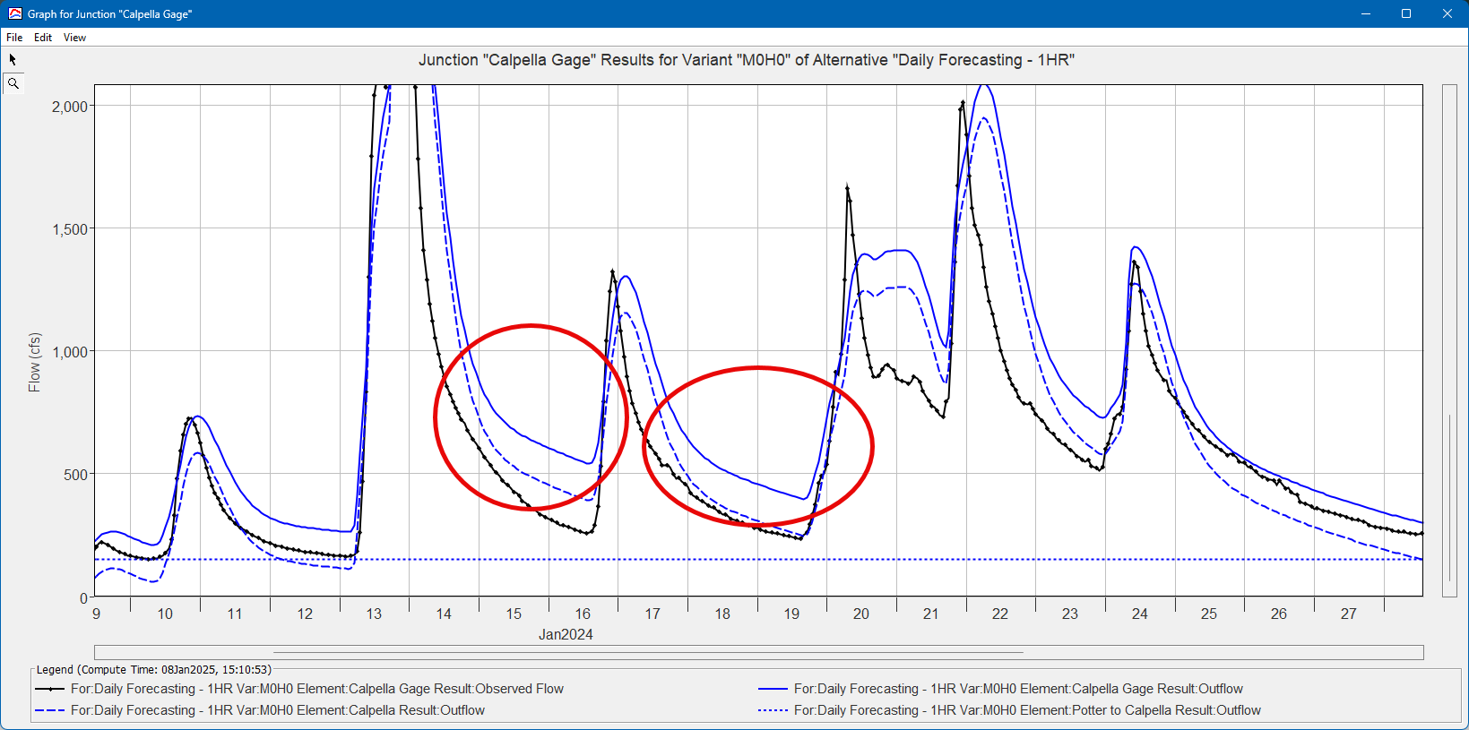 
    
11. Open the Linear Reservoir Baseflow tab in the Combined Parameter Editor. Change the GW 1 fraction to 0.2 and the GW 2 fraction to 0.3 for the Coyote zone and rerun the simulation. As shown in the figure below, the baseflow response (GW1 and 2) improved. 
    
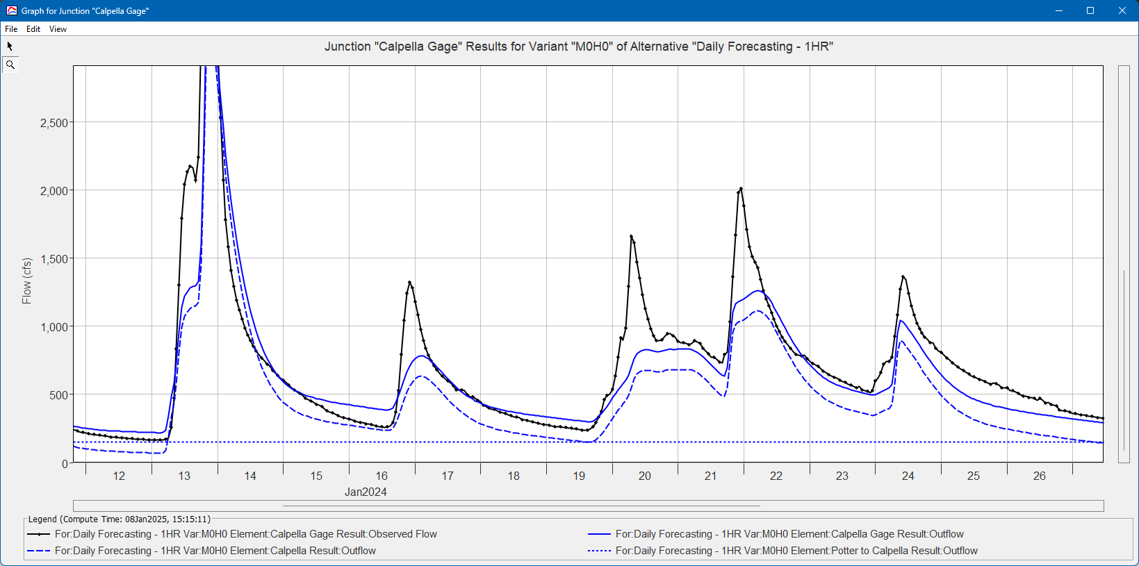
12. Go back to the Deficit Constant Loss tab in the Combine Parameter Editor and change the Constant Rate adjustment factor to *0.3 for the Coyote zone. Rerun the simulation. You should notice the Nash-Sutcliffe is 0.930, which is great, and the Percent Bias is -0.68%. The flow hydrograph at Calpella Gage looks great, but as shown below, the computed reservoir stage is high compared to the observed stage. 
    
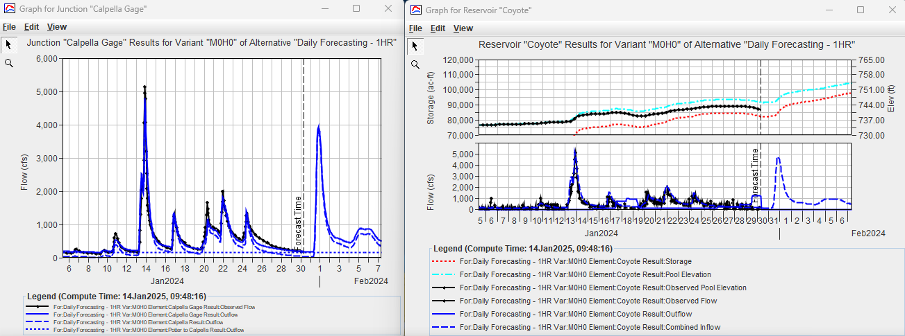
    At this point, we need to take one final sweep through the baseflow fraction parameters and reduce the amount of total runoff volume flowing into Coyote reservoir. In this case, we are slightly sacrificing the accuracy of results at the Calpella Gage location to improve simulated inflow into Lake Mendocino. Change the GW 1 fraction to 0.1 and GW 2 fraction to 0.15 for the Coyote Zone. Rerun the simulation. Results should be similar to those shown below.  

The following figure shows a plot from the Coyote Reservoir Elevation tab within the CAVI Dashboard.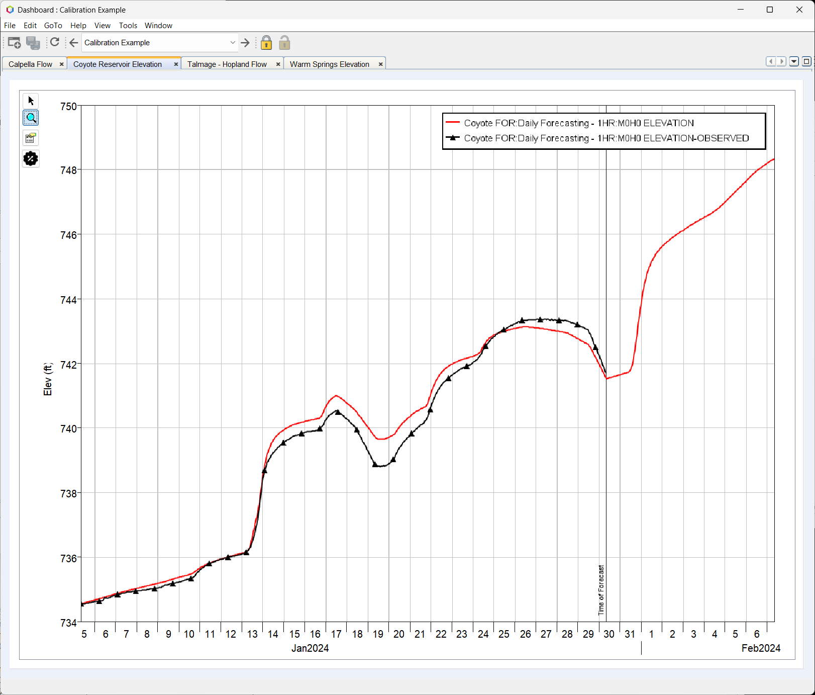

What is the Percent Bias and Nash-Sutcliffe for simulated and observed reservoir elevation for the Coyote reservoir? What happened to the Percent Bias and Nash-Sutcliffe at Calpella Gage?

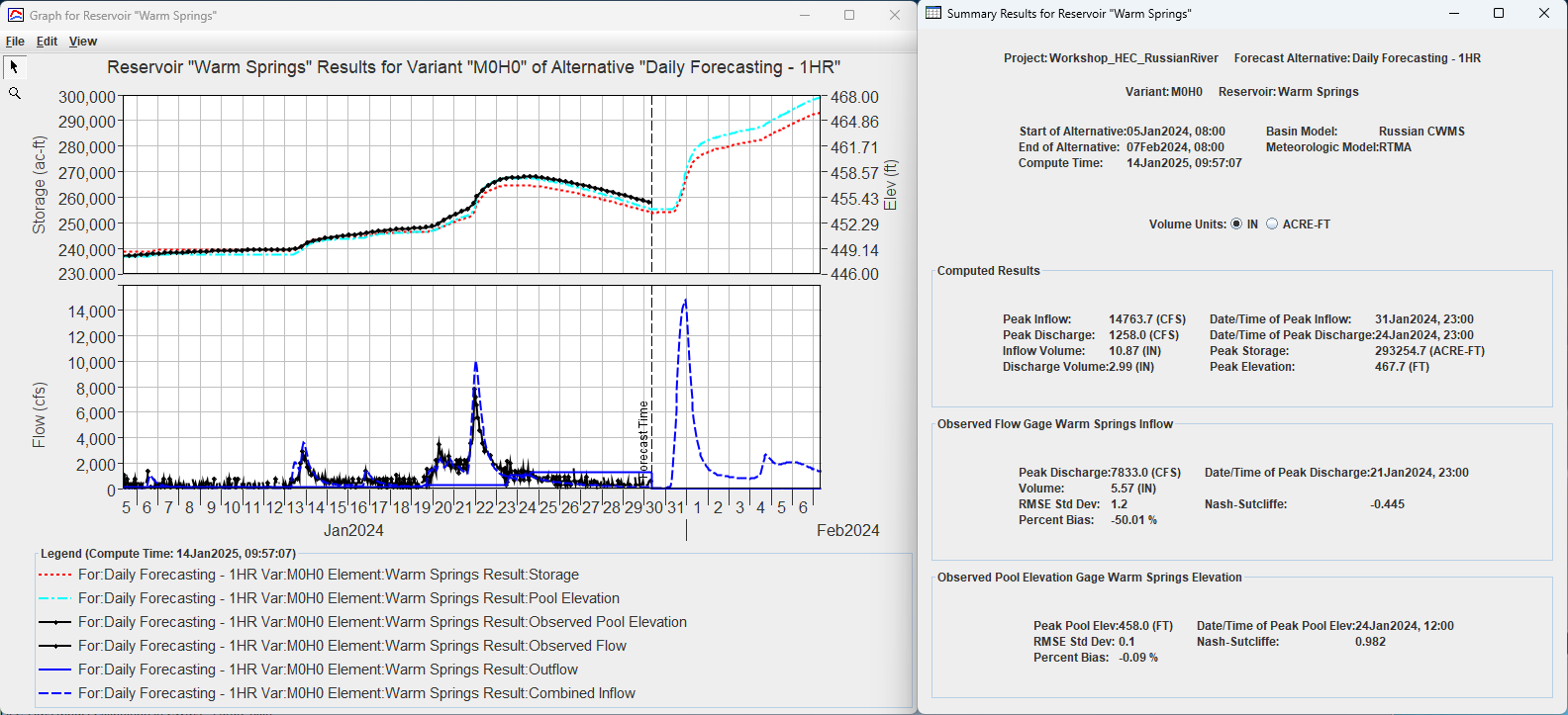
Take what you learned above and calibrate the model to accurately reproduce inflows for the Warm Springs reservoir. Only adjust the Initial Loss and Constant Rate Deficit and Constant Loss parameters and the GW 1 and GW 2 Fraction Linear Reservoir Baseflow parameters. Use the Combined Parameter Editor and adjust the zonal override table for the Warm Springs zone. Do not forget to select the Warm Springs computation point at the bottom of the Combined Parameter Editor. This simulation run time should be short because precipitation-runoff processes are only being computed for the Lake Sonoma subbasin. 

What were the final parameter values for the Lake Sonoma subbasin?

What is the Percent Bias and Nash-Sutcliffe for simulated and observed reservoir stage for the Warm Springs reservoir?