Tutorial Data

CWMS_EFP.zipDownload and unzip this file. CWMS 3.4.1 was used to create the workshop files and instructions.

Objectives

The overall goal of this tutorial is to provide a step-by-step guide to acquiring ensemble streamflow data shared by the National Weather Service (NWS), setting it up in CWMS CAVI, running simulations using ensemble forecast datasets, and reviewing the results. The steps described in the tutorial have already been completed within the attached project, you can reference the model as you read through the steps.

Upon completion of this tutorial, you will be able to:

1. Acquire meteorological gridded data from the National Blend of Models (NBM) (link here) and ensemble forecast streamflow data from the National Weather Service River Forecast Center (link here) in your region.
2. Set up CAVI to forecast rainfall-runoff responses: (i) considering only the HEC-HMS model –without ensemble and (ii) considering ensemble forecast streamflow as input at a selected forecast location.
3. Forecast streamflow and reservoir operations using the National Blend of Models gridded precipitation data and the ensemble forecast streamflow, selecting any ensemble member of interest, such as minimum volume, maximum volume, average volume, and percentile volume over a specified number of days.
4. Review the results and customize ensemble plots.

Background

The accuracy of streamflow predictions in any hydrologic model depends on several key factors. These include the type of model selected (e.g., lumped, distributed, or database-driven), the input variables and parameters used, and the accuracy of boundary condition (precipitation) measurements used by the model. Additionally, the accuracy of initializing hydrologic conditions and the accuracy of weather forecasts play crucial roles in determining the model’s predictive performance.

Often, model input climatic or meteorological variables, such as temperature, precipitation, wind speed, and solar radiation, are not entirely accurate. This inaccuracy can result from multiple sources, including the chaotic nature of the atmosphere or measurement errors (e.g., human errors or the spatial and temporal variability of weather parameters within a watershed). Moreover, any model prediction is inherently associated with other uncertainties, such as model assumptions, parameter values, and algorithms considered while developing a model. As a result, most of the streamflow forecasts may deviate from the actual observations.

One effective way to address these uncertainties is using multi-value forecasts, rather than relying on a single-value prediction. This approach, known as ensemble forecasting, generates a range of potential outcomes, offering a more comprehensive view that accounts for various uncertainties. Instead of producing a single deterministic forecast, the ensemble (probabilistic and multi-model) approach involves running multiple simulations. This method provides valuable insights to support water resources management decisions, such as reservoir operations and flood risk management.

The Ensemble Forecast Processor (EFP) is a plugin available in CWMS 3.4.  The intended application of this tool is to generate various statistical metrics from ensemble flows at specified locations in a watershed in order for forecasters to evaluate how those metrics influence other model alternatives in the forecast. For example, an HEC-ResSim alternative could use a statistical metric, such as minimum volume, maximum volume, average volume, and any percentile volume over a specified number of days, to evaluate and decide reservoir releases. See also the EFP Manual for more discussion, link here.  

Developing an ensemble forecast begins with meteorological data and involves further evaluating the hydrologic model values. The ensemble forecasting data in this tutorial were acquired from the California Nevada River Forecast Center (CNRFC), link here. The CNRFC ensemble streamflow forecasts, derived from statistical analysis of past forecast skill, reflects only meteorological uncertainty, without accounting for hydrologic uncertainty. 

Tutorial Data

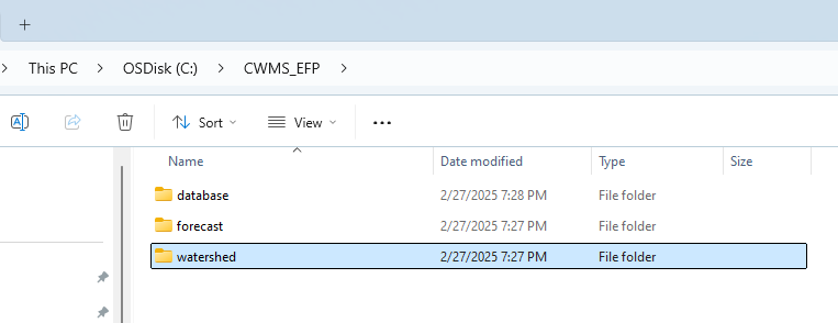
This tutorial includes models of a portion of the Russian River Basin in California. Therefore, forecasts using the model in this tutorial will not be comparable with other similar tutorials presented in the CWMS resources. As shown below, you must unzip the watershed, forecast, and database folders to the C:\CWMS_EFP directory on your computer to easily run the example.  

Tasks: 

The three main tasks are:

1. Data Acquisition 
2. Configuring the Ensemble Forecast Processer in CAVI
3. Running Ensemble Simulations, Reviewing Results, and Analyzing Ensemble Plots 

Task 1: Data Acquisition

1.1 Acquire meteorological gridded data from the National Blend of Models (NBM) Source

The gridded dataset applied here was pulled from the NBM dataset generated by NOAA. Users can find more information about how the NBM dataset is generated on NOAA’s website (link here). The gridded precipitation considered for this tutorial were acquired from Cumulus (link here). Cumulus is a USACE web service that provides gridded meteorological, observed and forecast, and hydrologic data across the United States. Multiple forecast datasets are available, NBM was chosen for this tutorial for example purposes only.

Users can follow all the standard steps outlined in CWMS Tutorial and Workshop resources (e.g., Setting Up a Cumulus Extract: link here), which are not repeated in this tutorial (see the figures below for reference). 

The figures below provide snapshots of the main steps required to acquire meteorological gridded data from the National Blend of Models source. Each orange arrow indicates the flow of operations, starting from the Setup tab and pointing towards the successive steps. If you look at the example project, you will notice an Extract Group named Cumulus has already been configured. 

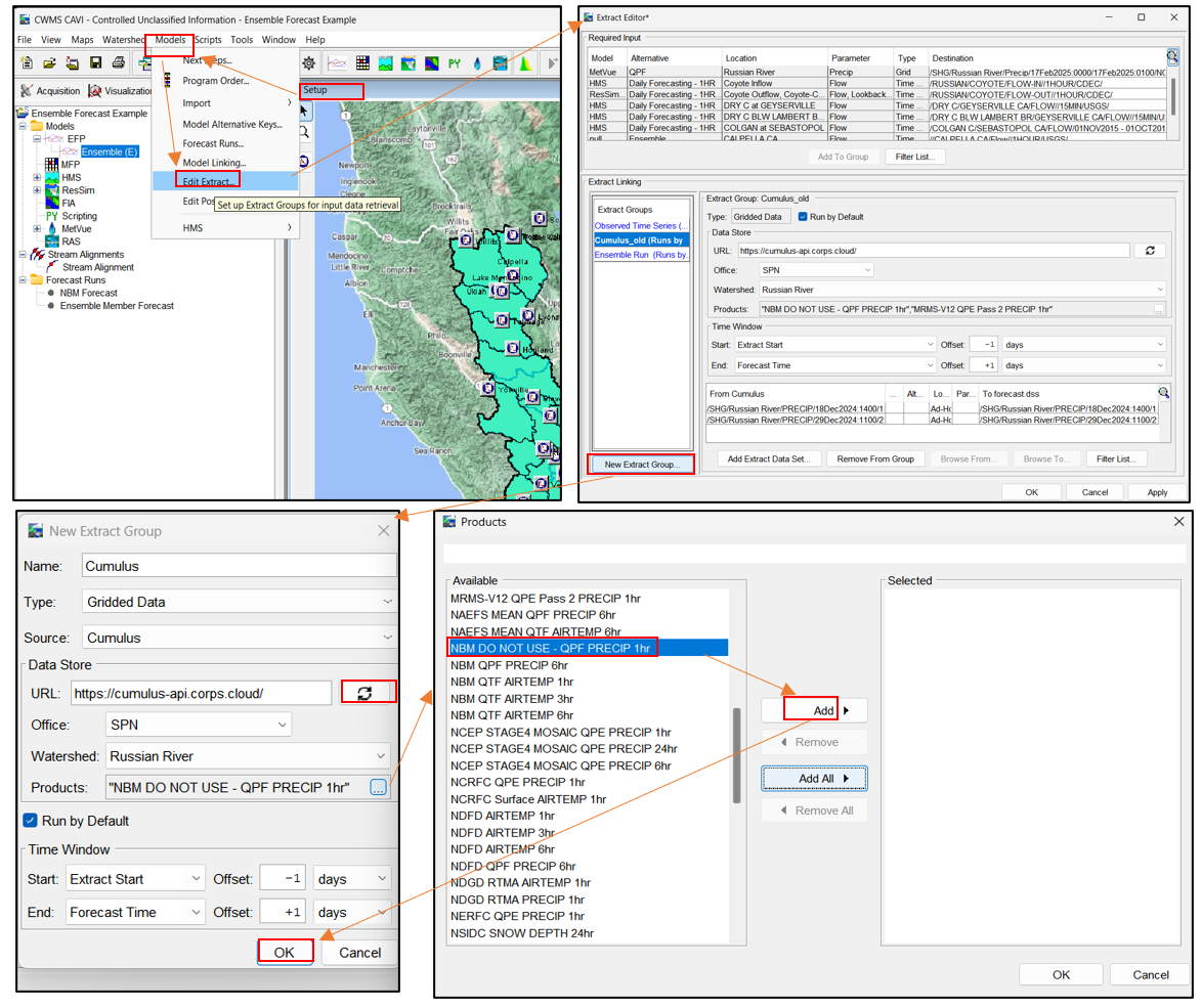
The figures below illustrate the steps followed to set up the Extract Editor and Extract Linking. 

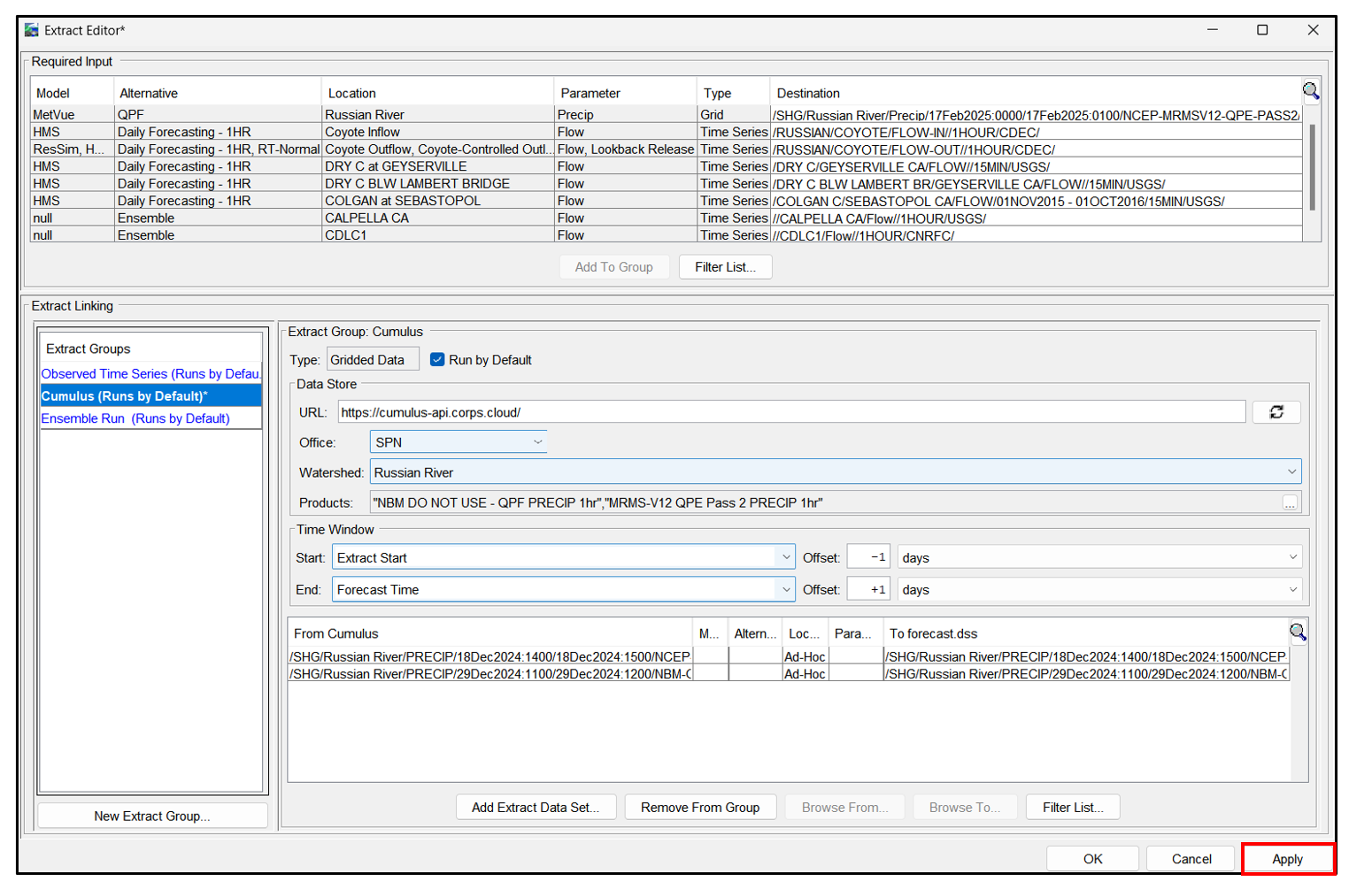
The following figure shows the Cumulus Extract Group after it was completed. The MRMS data set is used in the forecast lookback period and the NBM dataset is used in the forecast period. 

1.1 Acquire Ensemble Forecast Streamflow Data

1. Make sure that the Ensemble Data Acquisition Script (e.g., a file named "ESP_Import_russain.py" in this example) is available in the CAVI Script Editor.
2. If it is unavailable, find the script file and add it to the Script Editor. For information on how to set up a Script in CAVI, check related resources, such as "Set Up a Plot Script" in the CWMS workshop (link). The figure below shows the ensemble script available for extracting the ensemble data.
   
3. This Ensemble Forecasting Script has three functions:
   1. Downloads data for each forecast point of interest for a specified time interval.
   2. Processes and stores ensemble time series data in the DSS file.
   3. Handle errors if data for a forecast location is unavailable.
      
      The script used for this example is custom for the CNRFC and Russian River watershed. The forecast locations / streamgage names specified in River Forecasting Center's source must match the names in the Script (see "line 41 -51" of the Script Editor, where streamgages names are updated). The Script will generate an error message if the streamgage name is incorrect or if the named streamgage does not have data available.
      
4. Test the script to ensure that the script Save/Run operation is successful (see first figure below), and that data are stored in the designated “database” folder (e.g., see second figure below and file name: "C\CWMS_EFP\database\CNRFC_ensembles.dss"). It is noted that the script automatically downloads forecasted data for a specified river basin and streamgage, typically covering a month-long period starting from the day of running the script. Users can only modify the time window (i.e., the start and end dates) only by hardcoding the script. The script was run for this example, the time window that data was gathered was 18 December, 2024 - 17 January, 2025 (the ensemble dataset represents a forecast made on December 18, 2024).
    
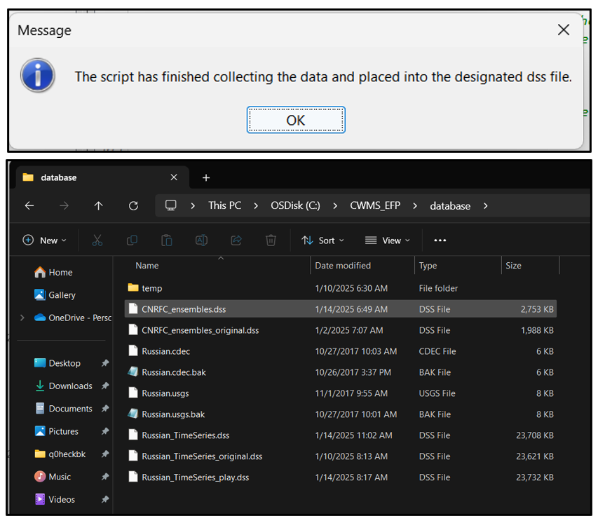
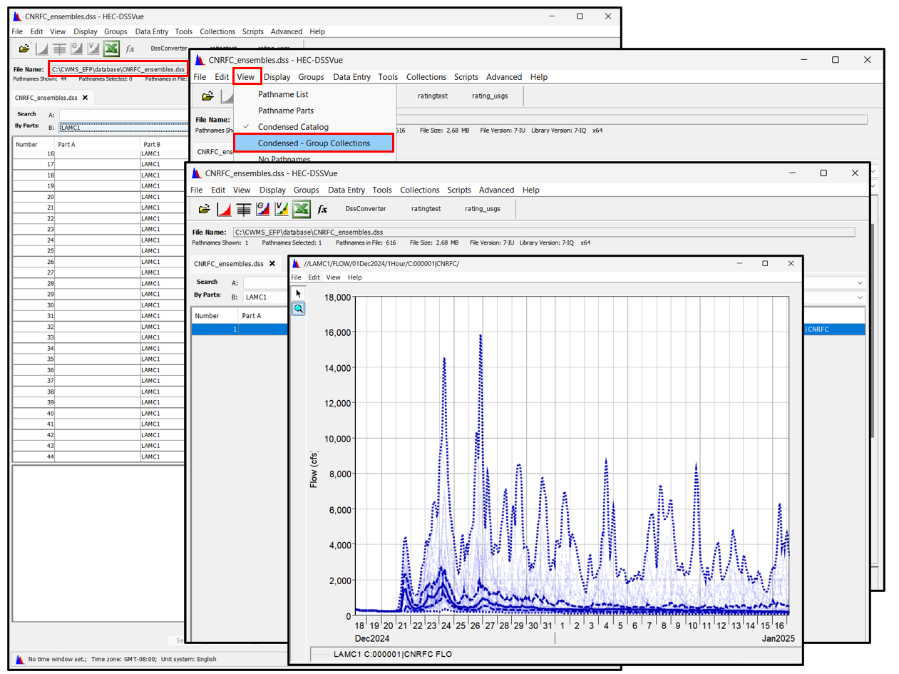
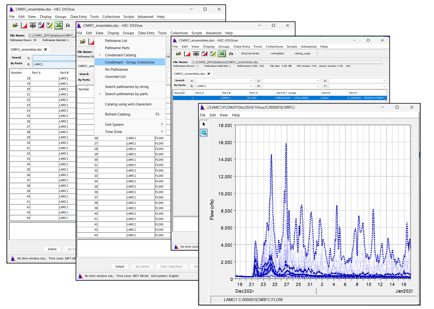
5. Go to the "database" directory and open the "CNRFC_ensembles.dss" HEC-DSS file. Select "Condensed - Group Collection" from the "View" menu and plot the downloaded ensemble streamflow data to verify that the input data is available. The following figure shows all forecast flow ensemble members for the LAMC1 location. 
   

Task 2: Setting up Ensemble Forecast Processor in CAVI

The EFP, a plugin available in CWMS 3.4.1, functions like any other program within the CAVI interface. To set up the EFP in CAVI, we need to create a new EFP alternative and complete the required CWMS modeling setup (these steps have already been completed in the example project). This includes defining the program order, setting model alternative keys, creating forecasting run alternatives, configuring model linking, and setting up extract lists.

2.1 Create a new EFP Alternative

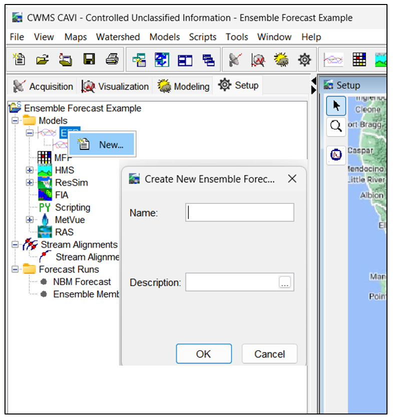
Navigate to the Setup tab, right-click on EFP, and select New to create a new alternative. A window of “Create New Ensemble Forecasting Processor Alternative” will appear. As shown below, enter a name for the alternative and add a description as needed.

2.2 Input Settings

Configure Input and Output Settings for the newly created Ensemble Forecast Processor. We can edit Name, Description, Input, and Output Settings by right clicking the created Ensemble alternative and selecting the Edit option. Navigate to the Input Settings, which consist of two tabs: LookBack and Forecast.

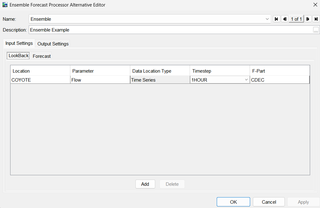
Entering data in the LookBack tab is only required if the Ensemble Member with "Closest Volume to Metric Compute" option is selected and if you want to merge observed time-series data from the LookBack Period with the ensemble member returned in the Forecast period. As shown in the figure below, we will merge observed streamflow from the lookback period with forecasted streamflow from one of the ensemble members for the forecast period. The observed streamflow will be linked to location information defined on the LookBack tab.

Input the following details when filling out the LookBack tab:

• Location – Enter the B-Part of the HEC-DSS Pathname. The name must match the B-part pathname for the record referenced and extracted into the Forecast.dss file. 
• Parameter – Enter the C-Part of the HEC-DSS Pathname (must match the associated parameter in the Forecast Period and Compute Location in Output Settings).
• Timestep – Select the timestep from the dropdown list (must match timesteps in the Forecast Period and Compute Location in Output Settings).
• F-Part – Enter the F-Part of the HEC-DSS Pathname.

2.2.2 Configure Forecast Tab

The Forecast Tab specifies forecast time-series data that the EFP will use in computations. To successfully compute an EFP alternative, you must enter at least one location in the Forecast Tab.

Click the Add button to add more data entries as needed. In this example, we are only using ensemble information for the inflow into Lake Mendocino. There are additional points in the watershed with ensemble time-series from the CNRFC; however, the total flow forecast is provided whereas the HEC-ResSim model of the Russian River watershed is configured to bring in local, or incremental, runoff hydrographs. Simulated results from the HEC-HMS model is used at downstream locations. The LAMC1 location corresponds to forecasted inflow into Lake Mendocino. 

Input the following details for each location of the Forecast tab:

• Location – Enter the B-Part of the HEC-DSS Pathname. The name must match the B-part pathname for the record referenced and extracted into the Forecast.dss file. 
• Parameter – Enter the C-Part of the HEC-DSS Pathname (must match the associated Parameter in the Compute Location under Output Settings, see Output Settings in next section).
• Timestep – Select the Timestep from the dropdown list (must match the Compute Location Timestep).
• F-Part – Enter the F-Part of the HEC-DSS Pathname (only include the identifier, e.g., CNRFC, excluding the collection portion, e.g., C:000001).

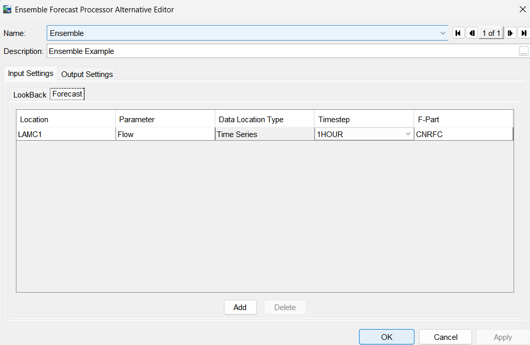
2.3 Output Settings

Navigate to the Output Settings tab, which allows us to define the desired output of the Ensemble Forecast Processor. The Output Settings consists of two separate tabs: Locations to Computer Metrics and Cumulative Volume Scalar Decision Metrics.

Locations to Compute Metrics Tab – Specifies locations where ensemble metrics will be computed and defines input data from the LookBack and Forecast time windows.

Cumulative Volume Scalar Decision Metrics Tab – Configures the metrics to be calculated for each forecast.

2.3.1 Configure Locations to Computer Metrics

The Locations to Compute Metrics tab lets us specify locations where the EFP will calculate statistical metrics. As shown in the following figure, only the Lake Mendocino inflow location was selected.

Similar to the Input Settings, complete the following for each location:

• Location – Name of the compute location (B-Part of the DSS output pathname).
• Parameter – The time-series parameter (C-Part of the DSS output pathname). Must match corresponding locations in the Lookback and Forecast periods.
• Timestep – Select the timestep (E-Part of the DSS output pathname). Must match corresponding locations in the Lookback and Forecast periods. 
• LookBack – Choose the record for the Lookback Period. The LookBack can be left "null" in two cases: (a) where the Ensemble Member with Closest Volume to Compute Metric not selected, or (b) the ensemble time series collection record selected in the Forecast Period covers the entire Time Window of the Forecast (from start of Lookback Period to the end of Forecast).
• Forecast – Select the ensemble time series record for computing metrics at this location.

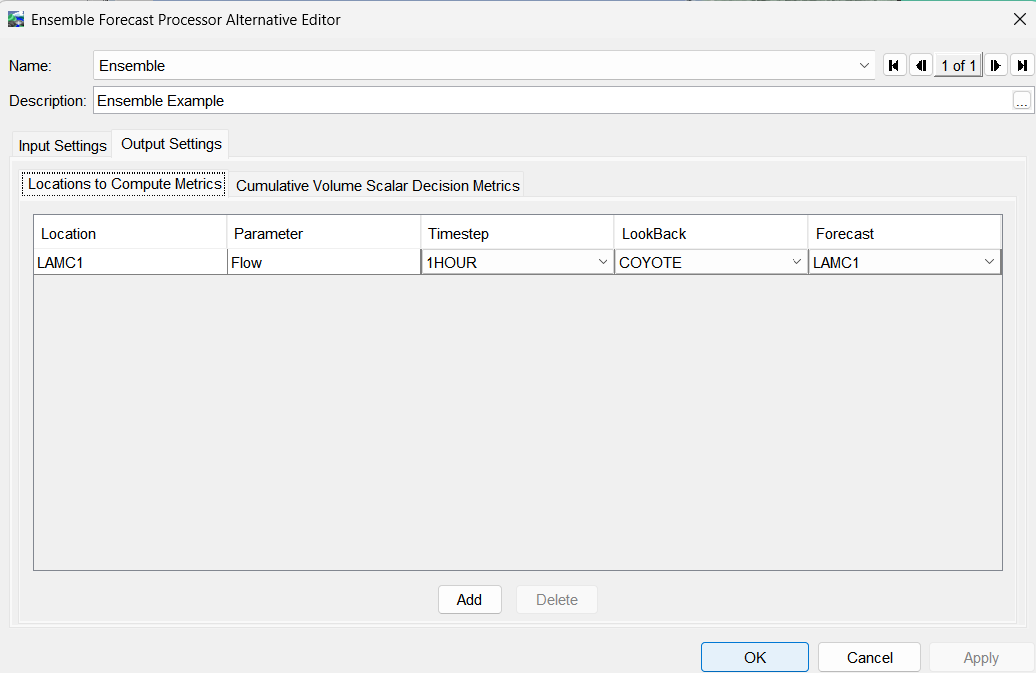
2.3.2 Cumulative Volume Scalar Decision Metrics

The "Cumulative Volume Scalar Decision Metrics" tab allows us to define metrics to be computed for each forecast. Follow the steps below to configure:

• Enter "Cumulative Volume" – Specify full days (e.g., 1, 3, 5) within the Forecast Time Window for the program to compute the cumulative volume. You can specify more than one volume duration.
• Enable Min, Max, Average, and Standard Deviation if needed. For example, when Min is selected, the program will compute and save the minimum volume from all ensemble members at the specified cumulative volume duration(s).
• Enter Percentiles – Input decimal values (e.g., 0.10, 0.50, 0.90) separated by commas. The program will compute and save volumes for the selected percentiles at the specified cumulative volume durations(s).
• Enable "Ensemble Member with Closest Volume to Metric" if you want to compute this additional metric. This feature identifies and saves the ensemble member (complete time-series) with the closest cumulative volume at user specified cumulative volume duration(s) to the selected metric (min, max, percentiles, average, and standard deviation). Cumulative Volume computations always begin at the Time of Forecast.  
• Press Enter to save data.

Notice in the following figure the option to save the Ensemble Member with the Closest Volume to Metric Compute is checked. Also, the 3-day cumulate volume was entered along with the 10th, 50th, and 90th percentiles. In this case, the program will create datasets that combine the observed inflow into Lake Mendocino for the Lookback period with the ensemble members that are closest to the 10th, 50th, and 90th percentile 3-day volume.  

2.4 Ensure CWMS Modeling Setup Completion

 Complete all the CAVI configuration required to run the CWMS model and any forecast simulations. Check other CWMS resources for details link. These steps were completed in the example project. 

2.4.1 Assign Model Alternative Keys

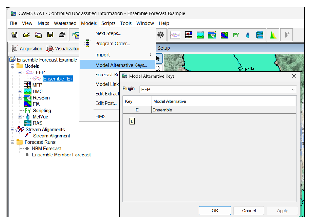
From the Setup Tab, go to Models > Model Alternative Keys, select a model from the Plugin drop-down menu, and enter a single-letter or number key in the left column. As shown in the figure below, a model key of "E" was used for the Ensemble EFP alternative. 

2.4.2 Define Program Order 

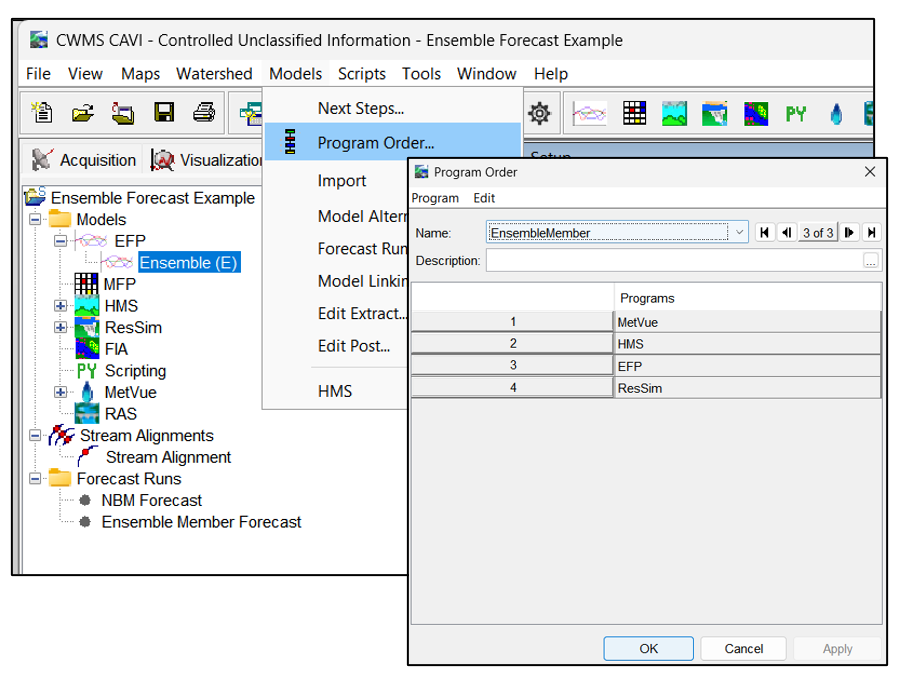
From the Setup Tab, go to Models > Program Order. Then, create a New program order from the Program menu. As shown below, make sure EFP is part of the compute sequence. 

2.4.3 Build Forecast Run Alternatives

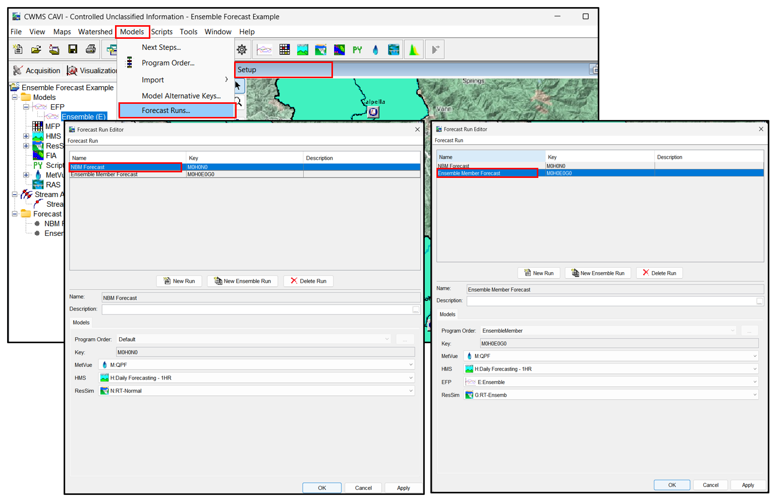
To build Forecast Runs, go to Models > Forecast Runs and click New Run from the Forecast Runs menu. Enter a Name and Description, select the Program Order, and then select the model alternatives (e.g., MetVue,  HEC-HMS,  Ensemble, HEC-ResSim). Click Apply to save.

The figures below show the Forecast Run Editors configured for both the NBM Forecast and the Ensemble Member Forecast.

2.4.4 Configure Model Linking

In CAVI forecasting, models must know their input source, either from a preceding model in the compute sequence or an external source like the extract list, which is managed using the Model Linking Editor.

In the Setup tab, go to Models > Model Linking to open the Model Linking Editor. Select the Forecast Run and name of the Model Requiring Input. Ensure the model receives correct observed datasets and boundary conditions from model in the compute sequence. Click "Apply" when finished. 

The following figures show that the ResSim model alternative is linked to the EFP model alternative. The example is set up to pass observed inflow plus Ensemble forecast members computed by the CNRFC to the Lake Mendocino reservoir element in the ResSim model. The ResSim model is still linked to HEC-HMS output for locations downstream of Lake Mendocino.

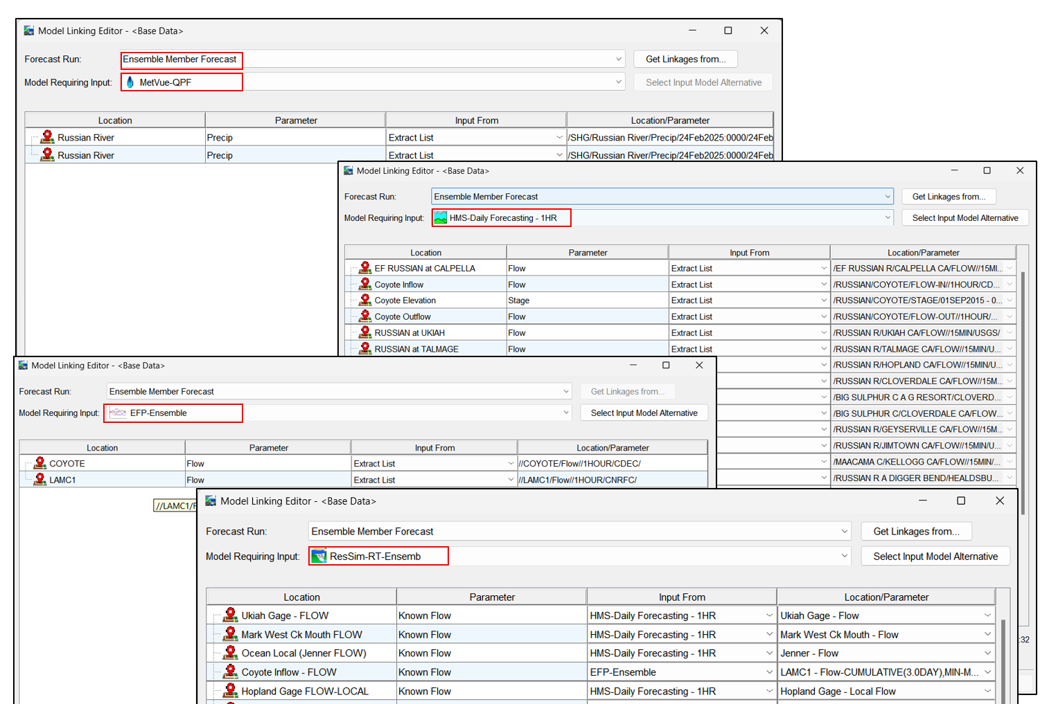
In the Model Linking Editor for "Ensemble Member Forecast," The COYOTE location requires input from "//COYOTE/Flow//1Hour/CDEC." This means you must ensure that the "forecast.dss" file does not contain an A-part in its DSS Pathname. The A-Part of the DSS Pathname must be blank for the computation to run successfully (see the figure below).

2.4.5 Configure Extract Lists

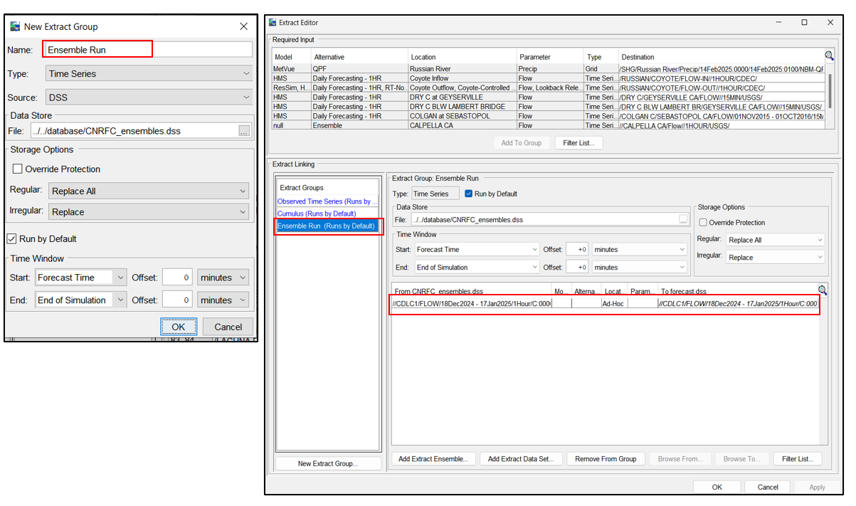
The Extract List in CAVI specifies where to retrieve data and how to extract it into the "forecast.dss" file. The forecast.dss file is single HEC-DSS file that all models can access for reading and writing during forecast simulations. Follow the standard steps to configure the Extract List, such as "Create a New Time Series Data Extract Group" and "Configure the Extract List." For more information, refer to other CWMS tutorials or workshop resources.

The following figure shows the extract list created to bring in the ensemble dataset into the "forecast.dss" file. 

Task 3: Run the Ensemble Simulations, Review the Results and Ensemble Plots

3.1 Run the Ensemble Simulations and Review the Results

The results presented in the example are based on the Coyote Junction upstream of Lake Mendocino and the Talmage Junction downstream of Lake Mendocino (see the figure below).

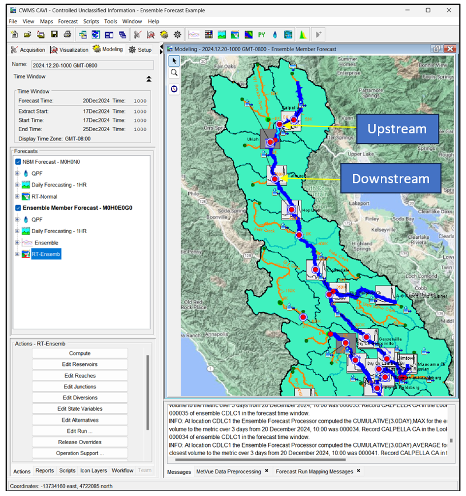
The following two simulation scenarios are considered: "NBM Forecast" and "Ensemble Member Forecast". The NBM Forecast has a standard compute sequence where MetVue and HMS are used to generate flow forecasts which are used by the ResSim model. The Ensemble Member Forecast uses individual ensemble members provided by the CNRFC at Lake Mendocino. The Ensemble Member Forecast uses MetVue and HMS forecast flows for locations downstream of Lake Mendocino. As you will see, you can easily configure the EFP simulation to select different ensemble members to get an idea of the uncertainty in the forecast as provided from the NWS River Forecast Centers. 

3.1.1 Normal Simulation

The standard steps were followed to create a CWMS forecast. MetVue, HEC-HMS, and HEC-ResSim are used to simulate rainfall-runoff responses both upstream and downstream of the reservoir using the National Blend of Models gridded precipitation dataset.

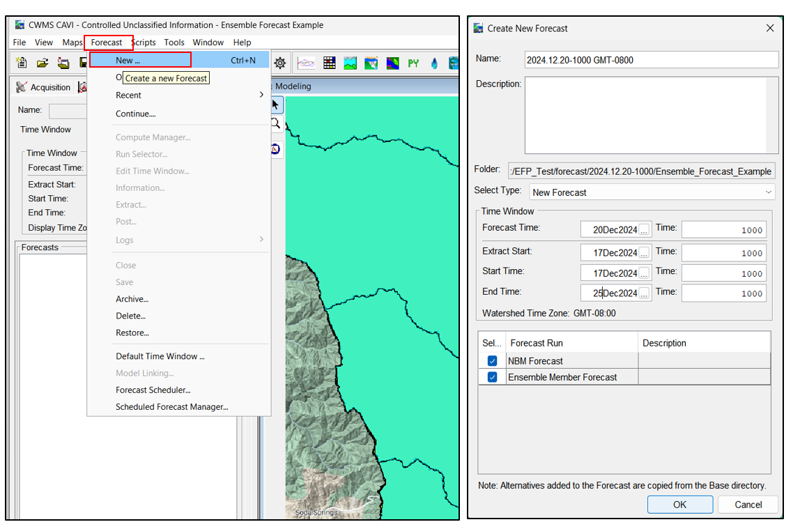
1. As shown below, A new forecasts was created for the NBM Forecast and Ensemble Member Forecast Simulations. 
   
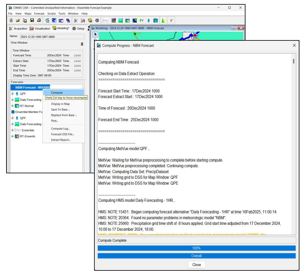
2. Open the 2024.12.20-1000 forecast, and compute the “NBM Forecast-MoHoNO” forecast. As shown below, the simulation should run to completion with no issue.
   
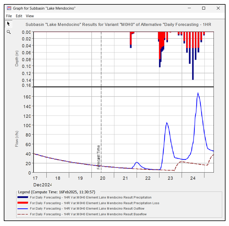
3. Evaluate whether the precipitation and other components of runoff are reasonable in the subbasins of interest using HEC-HMS. It is expected that all models are properly calibrated in the lookback period. As shown in the figure below, there is only baseflow in the lookback period before a few waves of precipitation in the forecast period. 
   
4. View the HEC-ResSim results plots upstream and downstream of Lake Mendocino by right-clicking on the "Plot" option for the Coyote and Talmage Junctions.  The figure below shows inflows into the reservoir and the  outflow hydrograph for the NBM precipitation forecast.
   

3.1.2 EFP Simulation

For this illustration, we performed an EFP simulation by selecting a single EFP trace as input at the Coyote Junction and running the simulation to evaluate the model's response at downstream locations. You can select any combination of single or multiple locations when using ensemble forecast information; however, you must use local runoff, not total runoff, downstream of reservoirs in your ResSim models since local runoff was setup when linking the ResSim and HMS model alternatives. Once a simulation using an ensemble member is complete, we will compare the results from the Ensemble Member and NBM forecasts to assess variability in the forecast.

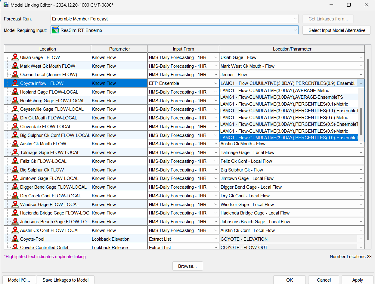
1. Compute the “Ensemble Member Forecast” forecast run. Before starting the computation, ensure that the CAVI setup is complete, and that "Model Linking" is correctly configured for the selected ensemble member. For example, in the following figure, the ensemble member closest to the 3-day 10th percentile volume is linked to the ResSim Model Alternative.
   
   
2. After a successful Compute, review the messages generated in the Compute Progress window to verify that the dates and other information are correct and as expected.
   
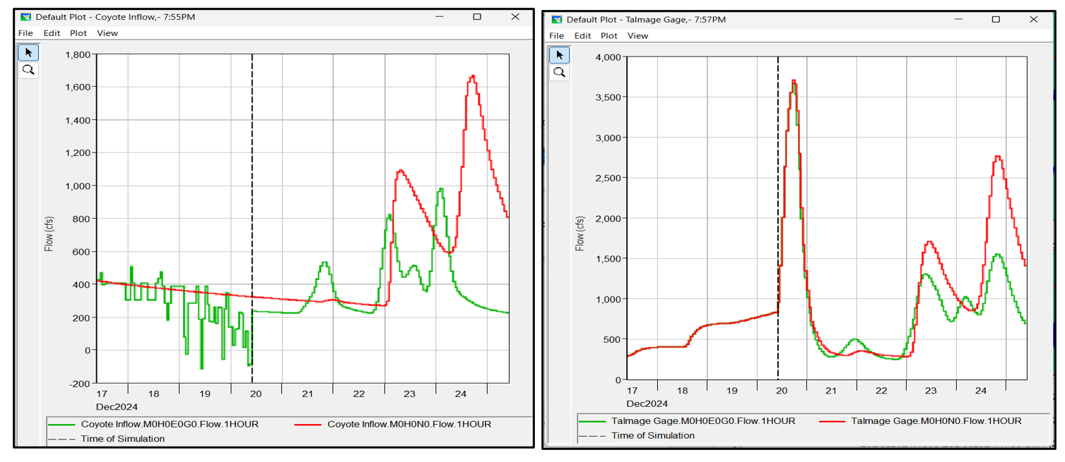
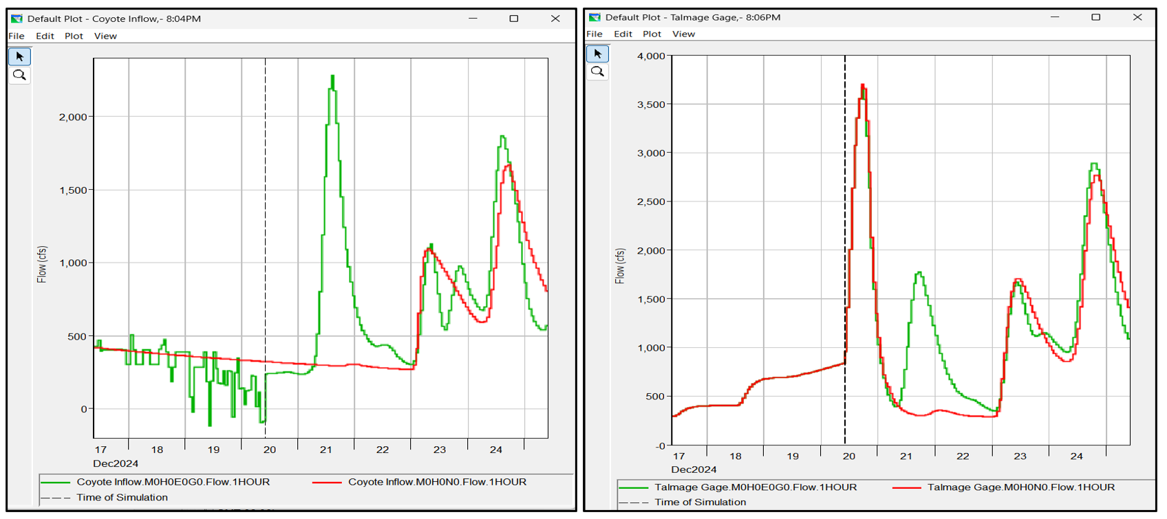
3. View the HEC-ResSim results plots upstream and downstream of Lake Mendocino by right-clicking on Coyote Junction and Talmage Junction. Note that we are also comparing these results with the NBM Forecast scenario by ensuring the NBM Forecast run is also active. The figures below present a comparison between the NBM forecast (red line) and the ensemble member closest to the 10th percentile 3-day volume of the ensemble forecast (green line).
   
4. It it easy to run other ensemble simulation scenarios. The figure below show the Model Linking Editor where the ensemble member closest to the 50^th percentile 3-day volume is selected. Choose the same EFP output and re-run the Ensemble Member Forecast simulation.
   
5. The figures below presents a comparative result between the NBM forecast (red line) and the ensemble member closest to the 50th percentile 3-day volume of the ensemble forecast (green line) for Coyote Junction and Talmage Junction. Notice the ensemble member picked up a large flood event on December 21 and the NBM forecast dataset did not include enough precipitation for this event to generate a similar response. 
   
6. The figure below show the Model Linking Editor and the ensemble member closest to the 90^th percentile 3-day volume is selected. Make the same selection in your model and rerun the forecast.
   
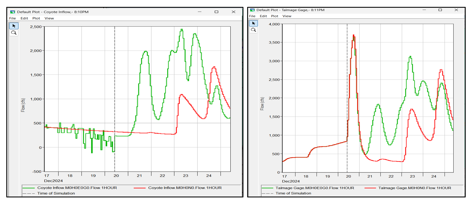
7. Similar to the 10th and 50th percentiles run, the figures below present a comparative result between the NBM forecast (red line) and the ensemble member closest to the 90th percentile 3-day volume of the ensemble forecast (green line) for Coyote Junction and Talmage Junction. Notice the ensemble member has much higher runoff than the NBM forecast. A large difference in ensemble datasets highlights the large uncertainty in forecasted streamflow. 
   
   

3.2 Evaluate Ensemble Plots

3.2.1 Evaluate downloaded Ensemble Streamflow data

As shown below, we can view all ensemble members in the downloaded ensemble file (e.g., "CNRFC_ensembles.dss") stored in the "database" folder. 

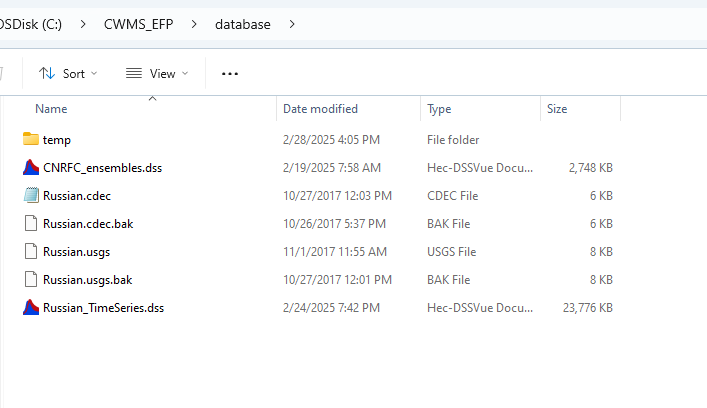
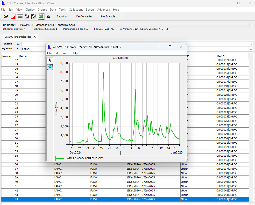
The file contains 44 ensemble members, and we can plot any of them using HEC-DSS (as shown below, the 44th ensemble member for the LAMC1 location is selected and plotted).

To view and plot all ensemble members, select Condensed-Group Collection from the View menu in HEC-DSSVue (as shown below). Note that collection plots are not accessible from the timeseries icons within the CAVI interface.

3.2.2 Evaluate a Simulated Percentile Member

We selected ensemble members that were closest to the 10^th, 50^th and 90^th percentile 3-day volumes for this example. If we would like to know which are the nearest members of those percentiles, we can check the log file generated during the ensemble forecast run. For example, the following figure shows ensemble members 00007, 00024, and 00018 are nearest to the 10th, 50^th and 90^th percentile 3-day volume.

3.2.2 Ensemble Viewer in CAVI

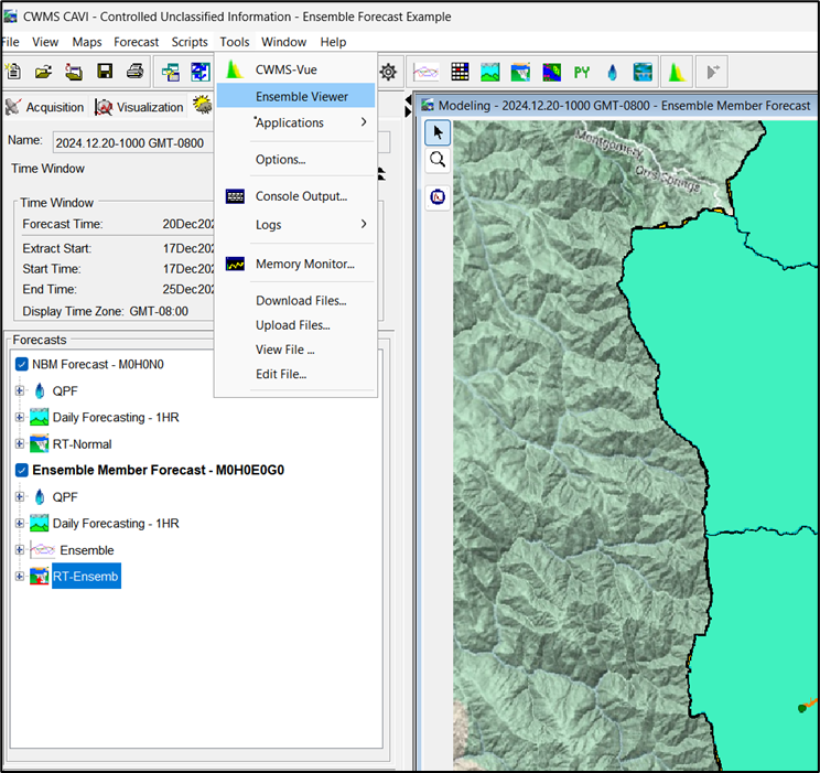
Ensemble visualization is also available using the Ensemble Viewer that is available from the CAVI “Tools” menu.

1. To check the ensemble results using CWMS CAVI, go to the "Tools" menu and select "Ensemble Viewer."
   
2. In the file explorer dialog, navigate to and select the "forecast.dss" file.
   
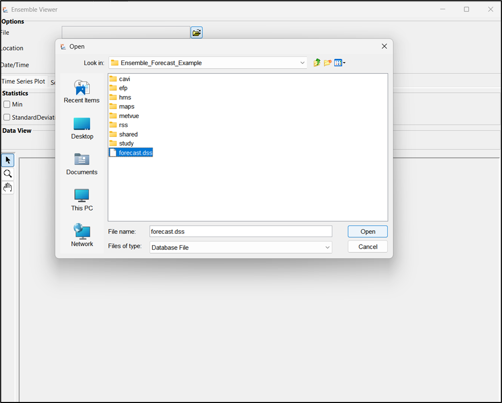
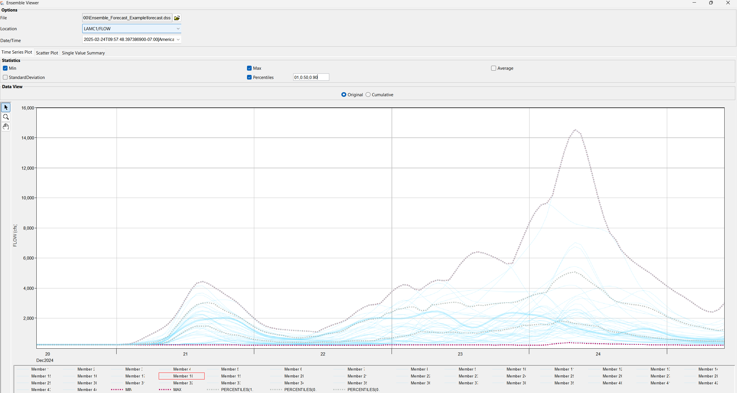
3. Once you open the selected file, the Ensemble Viewer will display the ensemble data. To view the selected junction or location, you can modify the default view. For example, in the Location tab, use the dropdown menu to choose a station with available ensemble views. Select the desired statistics, such as Min, Max, or Percentiles (e.g., 10th, 50th, 90th). The legend will display the ensemble members, allowing you to select, highlight, and edit individual traces.