Download PDF
Download page Applying the Deficit and Constant Loss Method.
Applying the Deficit and Constant Loss Method
Return to Introduction to the Loss Rate Tutorials.
Last Modified: 2025-01-29 16:35:35.556
HEC-HMS version 4.13-beta.4 was used to created this tutorial. You will need to use HEC-HMS version 4.13-beta.4, or newer, to open the project files.
Download the initial project files here:
Note: The initial project file is the same for the Initial and Constant Loss Method, the Green and Ampt Loss Method, and the Deficit and Constant Loss Method tutorials. If you are completing all three tutorials, the files only need to be downloaded once.

Overview
In this tutorial you will apply the HEC-HMS Deficit and Constant loss method to a modeling application. Initial parameter estimates will be estimated using GIS information and the model will be calibrated through trial and error.
Background
The Deficit and Constant loss method is very similar to the Initial and Constant loss method in that a hypothetical single soil layer is used to account for changes in moisture content. However, the deficit and constant method allows for continuous simulation when used in combination with a canopy method that will extract water from the soil in response to potential evapotranspiration computed in the Meteorologic Model. Between precipitation events, the soil layer will lose moisture as the canopy extracts infiltrated water. Unless a canopy method is selected, no soil water extraction will occur. This method may also be used in combination with a surface method that will hold water on the land surface. The water in surface storage can infiltrate into the soil layer and/or be removed through evapotranspiration. The infiltration rate is determined by the capacity of the soil layer to accept water. When both a canopy and surface method are used in combination with the deficit constant loss method, the system can be conceptualized as shown below.
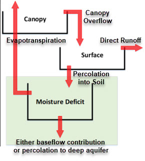
If the moisture deficit is greater than zero, water will infiltrate into the soil layer. Until the moisture deficit has been satisfied, no percolation out of the bottom of the soil layer will occur. After the moisture deficit has been satisfied, the rate of infiltration into the soil layer is defined by the constant rate. The percolation rate out of the bottom of the soil layer is also defined by the constant rate while the soil layer remains saturated. Percolation stops as soon as the soil layer drops below saturation (moisture deficit greater than zero). Moisture deficit increases in response to the canopy extracting soil water to meet the potential evapotranspiration demand. Parameters that are required to utilize this method within HEC-HMS include the Initial Deficit [inches or millimeters], Maximum Deficit [inches or millimeters], and Constant Rate [in/hr or mm/hr]. The Directly Connected Impervious Area [percent] is an optional parameter and can be specified by the user.
Estimate Initial Parameter Values
A Note on Parameter Estimation
The values presented in this tutorial are meant as initial estimates. This is the same for all sources of similar data including Engineer Manual 1110-2-1417 Flood-Runoff Analysis and the HEC-HMS Technical Reference Manual. Regardless of the source, these initial estimates must be calibrated and validated.
Initial Deficit
The Initial Deficit defines the volume of water that is required to fill the soil layer (to saturate the soil) due to the moisture state of the watershed at the beginning of the model simulation while the Maximum Deficit specifies the total amount of water the soil layer can hold. The Initial Deficit parameter is most often estimated using the product of the soil moisture state at the start of the simulation and an assumed active layer depth. However, this parameter must be calibrated using observed data, must be less than or equal to the Maximum Deficit, and must be specified as an effective depth (i.e. inches or millimeters).
In order to estimate an appropriate Initial Deficit, the antecedent conditions at the beginning of September 2018 must be investigated. Daily average humidity, daily precipitation accumulation, daily average temperature, and daily average wind speed for August 2018 are shown below.

Use the figure above and the following information to answer Question 1. Assume that the soil within the study area:
- Was completely saturated by rainfall on August 22, 2018 and
Requires approximately 14 days with no rain to completely dry under normal, summer conditions
Question 1: Estimate an initial deficit (in inches) for the study area at the beginning of September 2018.
A reasonable initial deficit is approximately 2 inches. However, this parameter must be calibrated using observed data.
Maximum Deficit
The Maximum Deficit is the driest a soil can become under the influence of gravity, evaporation, and transpiration. This parameter is typically estimated as the difference between the saturation storage of the soil and the wilting point storage over an assumed active soil layer depth. However, this parameter should be calibrated using observed data, must be greater than or equal to the Initial Deficit, and also must be specified as an effective depth (i.e. inches or millimeters).
Saturation Storage
Saturation storage refers to the amount of moisture that can be held within a soil column when all air bubbles have been forced out. This parameter is a function of the effective porosity. To estimate a representative effective porosity throughout the study area, Gridded Soil Survey Geographic (gSSURGO) data for Pennsylvania was obtained from the U.S. Department of Agriculture's Geospatial Data Gateway. Using GIS tools, surficial soil textures were then extracted from the gSSURGO data and are shown below. Also, the percent of the study area encompassed by each soil texture is shown in Table 1.
A tutorial describing how gSSURGO data can be obtained and formatted for use within HEC-HMS can be found here.

Table 1. Soil Textures Within the Study Area
Texture | % of Study Area |
|---|---|
| Sand | 0.1 |
| Loamy Sand | 0.0 |
| Sandy Loam | 3.7 |
| Loam | 17.1 |
| Silt Loam | 59.8 |
| Sandy Clay Loam | 0.0 |
| Clay Loam | 0.5 |
| Silty Clay Loam | 6.9 |
| Sandy Clay | 0.0 |
| Silty Clay | 0.0 |
| Clay | 0.9 |
| Bedrock | 10.7 |
These surficial soil textures can be used to estimate initial parameter values for nearly all loss methods within HEC-HMS, including the Deficit and Constant loss method. For instance, Rawls, Brakensiek, and Miller (1983) assembled data from thousands of soil samples located throughout the United States and related soil textures to various useful parameters. The effective porosity of various soil textures is shown in Table 2.
Table 2. Soil Textures, Effective Porosity, and Wilting Point, reproduced from Rawls, Brakensiek, and Miller (1983)
Texture | Effective Porosity |
|---|---|
Sand | 0.42 |
Loamy Sand | 0.40 |
Sandy Loam | 0.41 |
Loam | 0.43 |
Silt Loam | 0.49 |
Sandy Clay Loam | 0.33 |
Clay Loam | 0.31 |
Silty Clay Loam | 0.43 |
Sandy Clay | 0.32 |
Silty Clay | 0.42 |
Clay | 0.39 |
Use the Mahoning Creek surficial soil textures map, Table 1, and Table 2 to answer the following questions.
Question 2: What are the top five predominant soil textures throughout the study area?
Silt loam, loam, bedrock, silty clay loam, and sandy loam are the five most predominant soil textures (by area) throughout the study area. In fact, these five soil textures cover over 98% of the total study area. The remaining soil textures account for a very small percentage of the total area and can be disregarded.
Next, use Table 2 to answer the following question. Also, (conservatively) assume that bedrock has an effective porosity of 0 in3/in3.
Question 3: What is the effective porosity for the top five predominant soil textures found when answering Question 2?
Silt loam = 0.49 in3/in3, loam = 0.43 in3/in3, bedrock = 0 in3/in3, silty clay loam = 0.43 in3/in3, and sandy loam = 0.41 in3/in3.
Estimate an average (i.e. representative) effective porosity for the study area using your answers to the previous two questions. Don't spend too much time being overly precise; instead, quickly estimate the fraction of the study area that is encompassed by each predominant soil texture and multiply by the corresponding effective porosity. Once you've done that for each of the five predominant soil textures, sum the values.
Question 4: What is an average (i.e. representative) effective porosity for the study area?
Silt loam covers approximately 60% of the total area, loam covers approximately 17% of the total area, bedrock covers approximately 10% of the total area, silty clay loam covers approximately 7% of the total area, and sandy loam covers approximately 3% of the total area. Thus, (0.6 * 0.49 in3/in3) + (0.17 * 0.43 in3/in3) + (0.1 * 0.0 in3/in3) + (0.07 * 0.43 in3/in3) + (0.03 * 0.41 in3/in3) = 0.41 in3/in3.
Wilting Point Storage
Wilting point storage refers to the amount of water that is so tightly bound to soil particles that it cannot be evaporated or transpired. Technically, this parameter is defined as the water remaining within an initially saturated soil column when subjected to a sustained pressure of -15 bar (i.e. 217.5 pounds per square inch). Like effective porosity, this parameter can also be estimated using surficial soil textures. The wilting point storage of various soil textures is shown in Table 3.
Table 3. Soil Textures and Wilting Point, reproduced from Rawls, Brakensiek, and Miller (1983)
Texture | Wilting Point |
|---|---|
Sand | 0.03 |
Loamy Sand | 0.06 |
Sandy Loam | 0.10 |
Loam | 0.12 |
Silt Loam | 0.13 |
Sandy Clay Loam | 0.15 |
Clay Loam | 0.20 |
Silty Clay Loam | 0.21 |
Sandy Clay | 0.20 |
Silty Clay | 0.25 |
Clay | 0.27 |
Use the Mahoning Creek surficial soil textures map, Table 1, Table 3, and your answers to the previous questions to answer the following question.
Question 5: What is an average (i.e. representative) wilting point storage for the study area?
Silt loam covers approximately 60% of the total area, loam covers approximately 17% of the total area, bedrock covers approximately 10% of the total area, silty clay loam covers approximately 7% of the total area, and sandy loam covers approximately 3% of the total area. Thus, (0.6 * 0.13 in3/in3) + (0.17 * 0.12 in3/in3) + (0.1 * 0.0 in3/in3) + (0.07 * 0.21 in3/in3) + (0.03 * 0.1 in3/in3) = 0.12 in3/in3.
Finally, assume an active soil layer depth of 24 inches and use your answers to the previous questions to answer the following question.
Question 6: What is an average (i.e. representative) Maximum Deficit for the study area?
This parameter can be estimated by taking the difference between the saturation storage and the wilting point storage over an assumed active soil layer depth. Thus, (0.41 in3/in3 - 0.12 in3/in3 ) * 24 inches = 7.0 inches. However, this parameter should be calibrated using observed data.
Constant Rate
The Constant Rate defines the rate at which precipitation will be infiltrated into the soil layer after the initial deficit has been satisfied in addition to the rate at which percolation occurs once the soil layer is saturated. Typically, this parameter is equated with the saturated hydraulic conductivity of the soil which is defined as the rate at which water moves through a unit area of saturated soil in a unit time under a unit hydraulic gradient. This parameter can also be estimated using surficial soil textures. The saturated hydraulic conductivity of various soil textures is shown in Table 4.
Table 4. Soil Textures and Saturated Hydraulic Conductivity, reproduced from Rawls, Brakensiek, and Miller (1983)
Texture | Saturated Hydraulic Conductivity |
|---|---|
Sand | 4.6 |
Loamy Sand | 1.2 |
Sandy Loam | 0.4 |
Loam | 0.1 |
Silt Loam | 0.3 |
Sandy Clay Loam | 0.06 |
Clay Loam | 0.04 |
Silty Clay Loam | 0.04 |
Sandy Clay | 0.02 |
Silty Clay | 0.02 |
Clay | 0.01 |
Use the Mahoning Creek surficial soil textures map, Table 1, Table 4, and your answers to the previous questions to answer the following question.
Question 7: What is an average (i.e. representative) saturated hydraulic conductivity for the study area?
Silt loam covers approximately 60% of the total area, loam covers approximately 17% of the total area, bedrock covers approximately 10% of the total area, silty clay loam covers approximately 7% of the total area, and sandy loam covers approximately 3% of the total area. Thus, (0.6 * 0.3 in/hr) + (0.17 * 0.1 in/hr) + (0.1 * 0.0 in/hr) + (0.07 * 0.04 in/hr) + (0.03 * 0.4 in/hr) = 0.2 in/hr.
Directly Connected Impervious Area
Directly connected impervious areas are surfaces where runoff is conveyed directly to a waterway or stormwater collection system. These surfaces differ from disconnected impervious areas where runoff encounters permeable areas which may infiltrate some (or all) of the runoff prior to reaching a waterway or stormwater collection system. Within HEC-HMS, no loss calculations are carried out on the percentage of the subbasin that is specified as impervious area; all precipitation that falls on that portion of the subbasin becomes excess precipitation and subject to direct runoff. Within this tutorial, a directly connected impervious area percentage of 0 will be assumed.
Modify the Existing HEC-HMS Project
Now that you've estimated initial parameters, begin modifying the existing HEC-HMS project.
- Open the Punxsutawney_Loss_Methods project and then open the Mahoning_DeficitConstant Basin Model.
- Select the Mahoning Creek subbasin element.
- On the Subbasin tab, change the Loss Method from None to Deficit and Constant.
- Select the Loss tab to open the Deficit and Constant Component Editor.
- Enter the initial deficit, maximum deficit, constant rate, and directly connected impervious area values that were estimated in the previous section. The Deficit and Constant Component Editor should resemble the figure below.

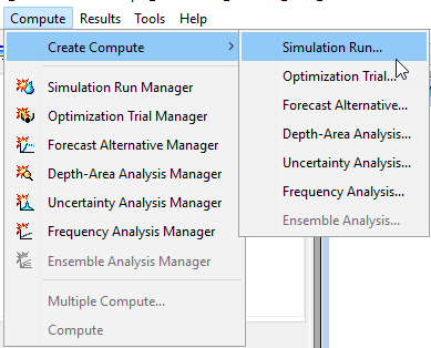
- Create a new simulation run by clicking Compute | Create Compute | Simulation Run.
- Name the new simulation run "Sept2018_DeficitConstant". Select Next>.
- Select the Mahoning Creek basin model. Select Next>.
- Select the MRMS meteorologic model. Select Next>.
- Select the September 2018 control specifications. Click the Finish button.
- Select the Sept2018_DeficitConstant simulation run from the Compute toolbar.

- Press the Compute All Elements button,
 , to run the simulation.
 - Select the Mahoning Creek subbasin element and click the the Result Graph button,
 , and the Summary Table button,
  .
. - Leave the summary table and plot open so you can see results change as you modify the loss method parameters. The observed streamflow is represented by the black dotted line and the model's computed streamflow is represented by the solid blue line.
- Notice that there is much less computed runoff than observed flow. This is confirmed within the Summary Table which shows large differences in observed and computed runoff volumes and peak flows, and poor statistical metrics.

- To better match the observed runoff, the Deficit and Constant loss method parameters must be calibrated.
Calibrate the Model
Calibrating a model to afford better agreement between computed and observed runoff oftentimes requires simultaneous changes to more than just one process (e.g. calibrate both loss and baseflow at the same time). However, within this tutorial, only the Deficit and Constant loss method parameters will be modified.
- Begin by modifying the loss parameters to approximately match the initiation of runoff.
- Change the Initial Deficit to 1 inch and the Constant Rate to 0.1 in/hr and rerun the simulation.
- The precipitation (dark blue) and precipitation loss (red) hyetographs for the Mahoning Creek subbasin element, in addition to the moisture deficit (magenta), are plotted below. Notice that the precipitation volume from the start of the simulation through approximately 09Sep2018 12:00 is used to satisfy the Initial Deficit (a volume of 1 inch). Afterwards, precipitation is infiltrated at a rate of 0.1 in/hr. When using a time step of 15 minutes, the effective rate is 0.025 inches / 15 minutes (i.e. 0.1 in/hr * 15 / 60). However, the moisture deficit begins to recover on 12Sep2018 at a rate that is equivalent to that which is specified within the MRMS Meteorologic Model. When using a time step of 15 minutes, the effective evapotranspiration rate for the month of September is 0.1167 inches / day (i.e. 3.5 inches / month * 1 month / 30 days). The moisture deficit that is recovered in between precipitation events must be satisfied before runoff initiates again. In this example, approximately 0.55 inches of moisture deficit is recovered and must be satisfied by precipitation on 17Sep2018.

- When looking at the Result Graph and Summary Table for the Mahoning Creek subbasin element, the computed hydrograph begins to rise at approximately the same time as the observed hydrograph, as shown below. However, the computed runoff volume (2.40 inches) is still much less than the observed runoff volume (4.4 inches) so further modifications are required.

- Continue modifying the loss parameters to approximately match the observed runoff volume.
- Change the Constant Rate to 0.05 in/hr and rerun the simulation.
- Notice that the computed runoff volume is now approximately equal to the observed runoff volume (4.36 vs 4.4 inches), as shown below. Also, the computed peak flow rate more closely matches the observed peak flow rate. However, the shape of the computed runoff hydrograph doesn't match the observed hydrograph shape on September 9th and 10th; in particular, the computed runoff is much greater than the observed runoff within those two days.

- To reduce the amount of runoff on September 9th and 10th, increase the Initial Deficit to 1.75 inches and rerun the simulation.
- Notice that the computed runoff volume is now less than the observed runoff volume (3.84 vs 4.4 inches), but the computed peak flow rate more closely matches the observed peak flow rate and the statistical metrics are very good, as shown below. Also, the shape of the computed hydrograph matches the observed hydrograph much better on September 9th and 10th.

- Continue adjusting the Deficit and Constant loss method parameters in an attempt to simultaneously best match the peak flow rate, runoff volume, and hydrograph shape. Record your RMSE Std Dev, Percent Bias, and Nash-Sutcliffe statistical metrics as you adjust model parameters.
- At this point, it should be apparent that simultaneously matching peak flow rate, runoff volume, and hydrograph shape can be difficult.
- For instance, the "double peak" runoff response within the observed results between September 9th - 11th is nearly impossible to recreate when using a single subbasin. This type of "signature" suggests two discrete pulses of runoff. To better match this response, two or more subbasins should be delineated.
Summary Questions
Question 8. What were the final Deficit and Constant loss method parameters and corresponding RMSE Std Dev, Percent Bias, and Nash-Sutcliffe statistical metrics for the calibrated model?
Using an initial deficit of 1.75 inches, a maximum deficit of 7 inches, and a constant loss rate of 0.04 in/hr offers an RMSE Std Dev, Percent Bias, and Nash-Sutcliffe statistical metrics of 0.3, -2.35%, and 0.896, respectively, as shown in Figure 10. However, these are by no means the only parameter combinations that can result in acceptable model calibration.

Question 9. Is it possible to reduce the computed runoff response on September 17th - 18th while not adversely affecting the computed runoff response on September 9th - 12th when using the Deficit and Constant loss method? If not, why?
YES! When using the Deficit and Constant loss method, the moisture deficit is continuously tracked. Also, when used in combination with a canopy method that will extract water from the soil in response to potential evapotranspiration computed in the meteorologic model, the soil layer will lose moisture as the canopy extracts infiltrated water.
However, this model uses the Recession baseflow method which is not connected to infiltrated volume and does not conserve mass. As a result, the calibrated Constant Rate value is very low to produce sufficient computed runoff volume.
It is important to consider how modeling methods interact when developing and calibrating a hydrologic model.
Download the final project files here:
Note: The final project file is the same for the Initial and Constant Loss Method, the Green and Ampt Loss Method, and the Deficit and Constant Loss Method tutorials. If you are completing all three tutorials, the files only need to be downloaded once.