Download PDF
Download page Viewing Model Results.
Viewing Model Results
Last Modified: 2025-01-27 08:40:26.592
Software Version
HEC-HMS version 4.13 beta 4 was used to create this tutorial. You will need to use HEC-HMS version 4.13 beta 4, or newer, to open the project files.
Project Files
If you are continuing from Creating and Computing a Simulation Run, you may continue to your current project files. Otherwise, download the initial project files here:

Overview
In this tutorial, you will view graphical, time-series, and summary results of subbasins, reaches, and junctions.
Steps
- Open the HEC-HMS project named Punxsutawney.
- Compute the simulation run: May 1996.
- To view the global summary table, click on the Results menu and select the Global Summary Table. Alternately, you can click the View Global Summary Table button,
 , on the toolbar; the button shows a table with a globe superimposed on it.
 - To view results for each basin model element, click on an element in the basin map with the right mouse button. A context menu is displayed with several choices including View Results. Under View Results you can see a graph, summary table or time-series table. You can obtain the same results by selecting the element, then clicking on the Results menu and selecting the appropriate option.
- To plot a graph for the Stump Creek subbasin, click on the Stump Creek subbasin in the basin map with the right mouse button, then click the View Results menu and select the Graph option.
The time-series shown in a graph are listed in the legend. The graph includes the incremental precipitation (blue in upper plot) and the precipitation loss (red in upper plot). Incremental precipitation is computed by the meteorologic model for each subbasin. The precipitation excess is the incremental precipitation minus the losses computed by the selected loss method. The graph also includes the baseflow (brown in lower plot) and the total subbasin outflow (blue in lower plot).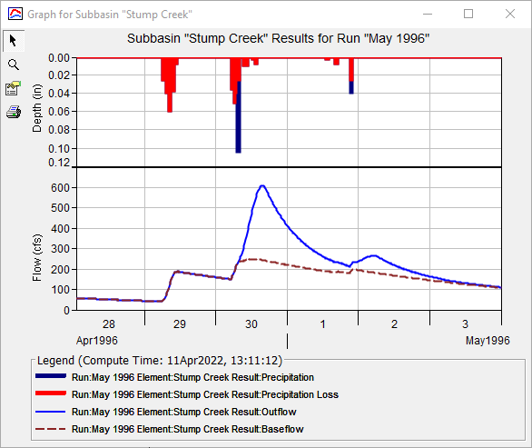
Summary statistics are automatically computed and shown in the summary table. Click on the Stump Creek subbasin in the basin map with the right mouse button, then click the View Results menu and select the Summary Table option.
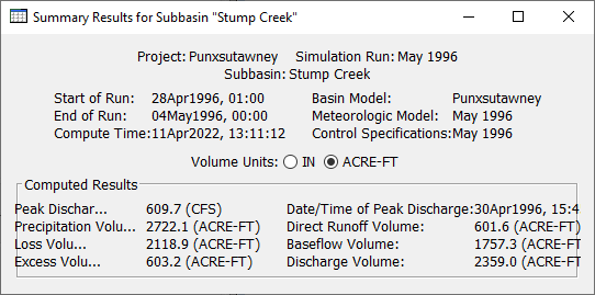
The summary table shows that the peak discharge is 609.7 cfs. The table also shows that the peak flow occurred on 30 April 1996 at 15:45 hours. When the table initially opens, it shows the total discharge volume is 1.525 inches as shown in the figure below. By clicking on the AC-FT radio button, the discharge switches units. The discharge volume is equivalent to 2350.0 AC-FT as shown in the second image below.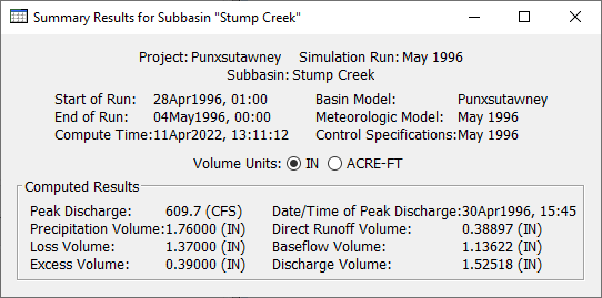
Question: What is the peak discharge for subbasin Mahoning Creek Local?1786.0 cfs
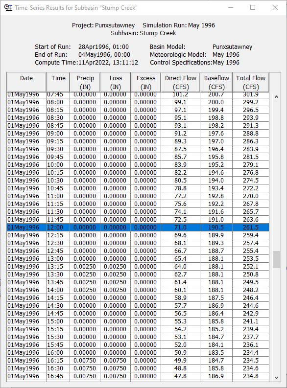
The computed discharge at a specific time is best determined from the time-series table for the element. Click on the Stump Creek subbasin in the basin map with the right mouse button, then click the View Results menu and select the Time-Series Table option. The image below shows a time-series results table.
Question: What is the baseflow for subbasin EB Mahoning Creek on May 1, 1996 at 12:00?333.1 cfs
- To plot results for Reach-1, as shown in the figure below, click on the Reach-1 reach in the basin map with the right mouse button, then click the View Results menu and select the Graph option. The time-series shown in a graph are listed in the legend. The graph includes the combined inflow to the reach (dashed blue) and also the computed outflow (solid blue). No matter how many elements connect to the upstream side of the reach, only the combined inflow is shown.

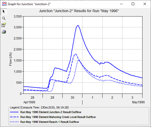
- To plot results for Junction-2, click on the Junction-2 junction in the basin map with the right mouse button, then click the View Results menu and select the Graph option. The time-series shown in a graph are listed in the legend. The outflow from the Punxsutawney Local subbasin (dashed blue) is shown along with the outflow from Reach-1 (dotted blue). If an observation time series is available at the location, a dotted black line is displayed. The total outflow is also shown (solid blue). All inflows into the junction from elements immediately upstream will be shown along with the total outflow, but no combined inflow is shown. Only graphs for junctions show the individual upstream inflows.
Summary
In this tutorial graphical, time-series, and summary results of subbasins, reaches, and junctions were demonstrated.
Continue to Viewing Observed Flow