Download PDF
Download page Task 2. Calibrate the Model for Water Years 1983-1992.
Task 2. Calibrate the Model for Water Years 1983-1992
Return to Task 1. Download, Import, and Manipulate Gridded Data
Last Modified: 2024-06-28 12:46:19.505
This tutorial demonstrates a process to calibrate an HEC-HMS model for a long term simulation.
Software Version
HEC-HMS version 4.12 was used to create this example. You can open the example project with HEC-HMS v4.12 or a newer version.
HEC-DSSVue version 3.2.3 is used to view and manipulate data within this example. You can download HEC-DSSVue here: https://www.hec.usace.army.mil/software/hec-dssvue/downloads.aspx.
Download the initial project files here:

Allotted Time
This task should take approximately 80 - 120 minutes to complete.
Introduction
Your goal in this task is to adjust model parameters within reasonable ranges to calibrate the model's performance in simulating snow water equivalent and inflow into Schafer Dam. Because we are using daily precipitation and temperature as boundary conditions, it will be challenging, or impossible, to simulate very good model performance when simulating every peak flow in the simulation time window. This would be true for other meteorologic datasets as well. Therefore, we will focus on evaluating performance using monthly average SWE and flow. Steps are included below showing how to convert HEC-HMS model results to monthly average values.
Model parameters have been mostly filled out for you. You are going to focus on the Constant Loss Rate, PX/Base Temperature, and Groundwater Fraction parameters when calibrating the model.
Complete Setup of the Model
- Open the project and become familiar with existing components.
- There is one basin model, named TuleRiver_Cal. Most parameters have already been defined in this basin model.
- The Livneh meteorologic model has been created. No precipitation, temperature or ET methods have been selected.
- Three control specification have been added. You will be using the CalibrationPeriod control specifications for this step. The simulation time window is 01 October 1982 through 01 October 1992. A 3-hour time step is used. This time step is too coarse for the size of watershed; therefore, there is some numerical attenuation in the transform calculations. No routing method was selected for the reaches because travel times are less than the simulation time step (lack of reach routing counteracts some of the numerical attenuation from the subbasin transform calculations).
- You will notice ATI meltrate and coldrate functions have already been defined for you.
- Flow, precipitation, temperature, and SWE data files are located in the projects data folder, ...\Schafer_Dam\data.
- Create a new discharge gage, named Schafer_Inflow, and link the data to the POR_Success_Q_In.dss file and //SUCCESS LAKE/FLOW-RES IN/01JAN1972 - 01JAN2022/1DAY/MERGE/ record. If you want to view the data, set the time window from 01 October 1972 through 01 October 2018.

- Create a new temperature gage, named Livneh, and link the data to the LivnehTemperature_WatershedAverage.dss file and //TuleRiver/TEMPERATURE/31Dec1914 - 30Dec2018/1Day/Average/ record. Save your project.
- Enter an elevation for the gage of 1215.6 meters. This is the average elevation of the watershed.
- Leave the reference elevation set to 9.99 meters.
Enter a latitude of 36.01594 decimal degrees. This is the latitude of the watershed centroid.

The General tab in the Program Settings editor lets you choose DEG Min SEC or Decimal Deg for displaying and entering latitude and longitude coordinates. Choose Decimal Degrees when working on this tutorial.
- Enter a longitude of -118.74223 decimal degrees. This is the longitude of the watershed centroid.

- Create a new snow water equivalent gage, named MFTuleR_S20_UofA, and link the data to the UofASWE_MFTuleR_S20.dss file and //MF_TULER_S20/SWE/01JAN1981 - 01JAN2011/1DAY/ENGLISH/ record. If you want to view the data, set the time window from 01 October 1982 through 01 October 2002.

- Create a new precipitation gridset, named Livneh_Precipitation, and link the data to the LivnehPrecipitation.dss file. Choose any of the precipitation grid pathnames.
- Create a new discharge gage, named Schafer_Inflow, and link the data to the POR_Success_Q_In.dss file and //SUCCESS LAKE/FLOW-RES IN/01JAN1972 - 01JAN2022/1DAY/MERGE/ record. If you want to view the data, set the time window from 01 October 1972 through 01 October 2018.
- Configure the Livneh meteorologic model.
- Choose the Gridded Precipitation, Interpolated Temperature, and Gridded Hamon methods.
- Open the Gridded Precipitation component editor and choose the Livneh_Precipitation gridset.
- Open the Interpolated Temperature component editor.
- Choose the Nearest Neighbor interpolation method (there is only one gage to interpolate).
- Select the Lapse adjustment method and enter a lapse rate of -3.0 DEG F/1000 FT.
- Select the Livneh temperature gage and enter a Radius of Influence to 50 miles (this will cover the entire watershed).

- Open the Gridded Hamon component editor. Notice the Hamon Coefficient has already been defined for you. Do not override the default value.
- Open the TuleRiver_Cal basin model.
- Set the Observed Flow for the ReservoirInflow junction element.
- Set the Observed SWE for the MF_TuleR_S20 subbasin element.
- Open the Deficit and Constant global editor and define a constant loss rate of 0.15 inches/hr as the initial value for all subbasins.
- Open the Gridded Temperature Index global editor and enter 32 Degrees F as the PX and Base temperature values for all subbasins.
- Open the Linear Reservoir global editor and enter a GW1 Fraction of 0.2, GW2 Fraction of 0.2, and a GW3 Fraction of 0.1 for all subbasins.
- Create a simulation run named CalibrationWindow. Select the TuleRiver_Cal basin model, Livneh meteorologic model, and the CalibrationPeriod control specifications.
- Run the simulation. The simulation should take about 45 seconds to complete.
Become Familiar with Model Results
- Open the Snowmelt plot for the MF_TuleR_S20 subbasin. Notice the simulated snow water equivalent is much lower than the "observed" snow water equivalent for most water years.

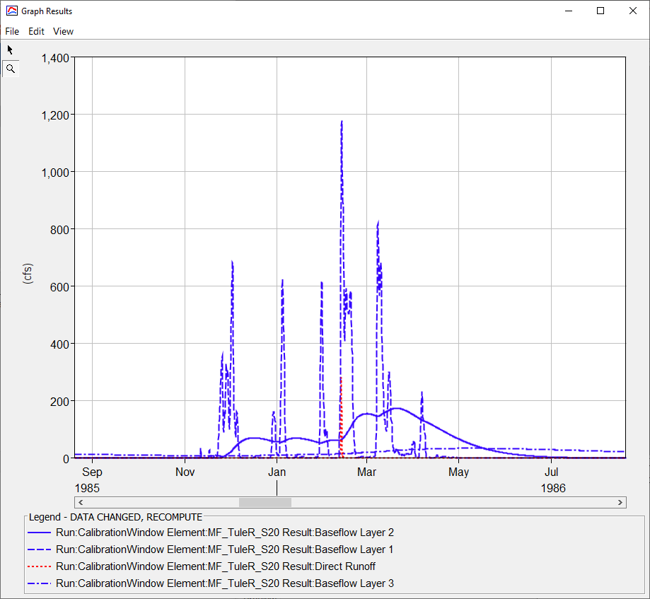
- Open the plot for the ReservoirInflow element and zoom into the 1986 water year as shown below. Notice the model is generating too much "peak" flow for many of the runoff events. The general trend for baseflow is good for this particular water year.

- Go to the Results tab of the Watershed Explorer and expand results for the MF_TuleR_S20 subbasin element. Notice all the results you have available to you.

- Hold down the control key and select the Direct Runoff, Baseflow Layer 1, Baseflow Layer 2, and Baseflow Layer 3 results. All results should plot in the preview pane. Then click the graph button in your toolbar to open a large plot of the selected results. You can also change the draw properties to help identify results. Notice in the figure below, direct runoff is a small portion of the simulated runoff. This result could indicate that the constant loss rate needs to be reduced.
- Select the Liquid Water at the Soil Surface and Moisture Deficit results. Notice how the moisture deficit increases during periods of no precipitation or snowmelt. The model is configured with a maximum deficit of 3 inches. No runoff is computed from the subbasin element until the deficit state variable is at a value of 0 inches.

- Select other results for subbasin elements to become familiar with the model.
- Hold down the control key and select the Direct Runoff, Baseflow Layer 1, Baseflow Layer 2, and Baseflow Layer 3 results. All results should plot in the preview pane. Then click the graph button in your toolbar to open a large plot of the selected results. You can also change the draw properties to help identify results. Notice in the figure below, direct runoff is a small portion of the simulated runoff. This result could indicate that the constant loss rate needs to be reduced.
- The following step shows you how to compare simulated and observed results at a different time scale than used to simulate the model. You can leave HEC-HMS open for this step.
- Open the MonthlyAverageResults spreadsheet. The CalibMonthlyAverageFlowResults and CalibMonthlyAverageSWEResults sheets have already been configured for you. All you need to do is paste in the monthly average flow and SWE results from HEC-HMS.
- Open HEC-DSSVue. Open the CalibrationWindow DSS file, this is the output DSS file HEC-HMS used to save all results from the basin model.
- As shown below, select the ReservoirInflow Flow result and the MF_TuleR_S20 SWE result. You may want to select View | Condensed Catalog to show the entire range of data.

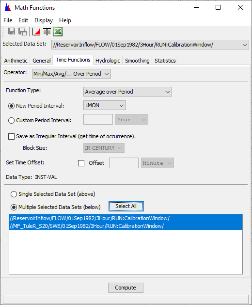
- Go to Tools | Math Functions.
- Select the Time Function tab.
- Choose the Average over Period function.
- Choose a New Period Interval of 1MON.
- Select the Multiple Selected Data Sets option, Select All records.
- Click Compute.
- Click the Save button and close the Math Functions editor.
- Click the Clear Selections button near the bottom of the window.
- As shown below, use the filter option to only display datasets with a 1Month E-part pathname.

- Select both records and choose the tabulate button. Copy and paste the monthly average SWE and Flow values into the MonthlyAverageResults spreadsheet, column E.
- The following figure shows the monthly average SWE results. Notice that the results from HEC-HMS are much lower that the observed SWE for this time period. Before adjusting Loss and Baseflow parameter you should adjust the temperature index PX and Base temperatures to improve the modeled SWE results.
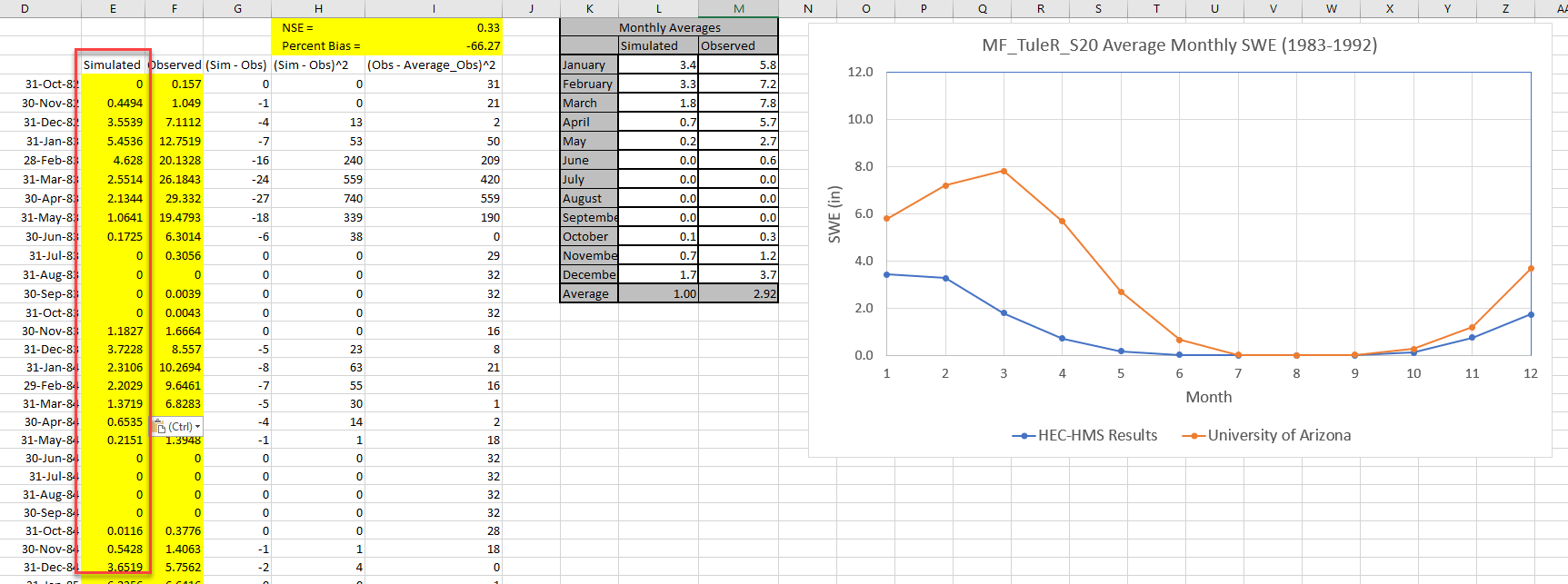
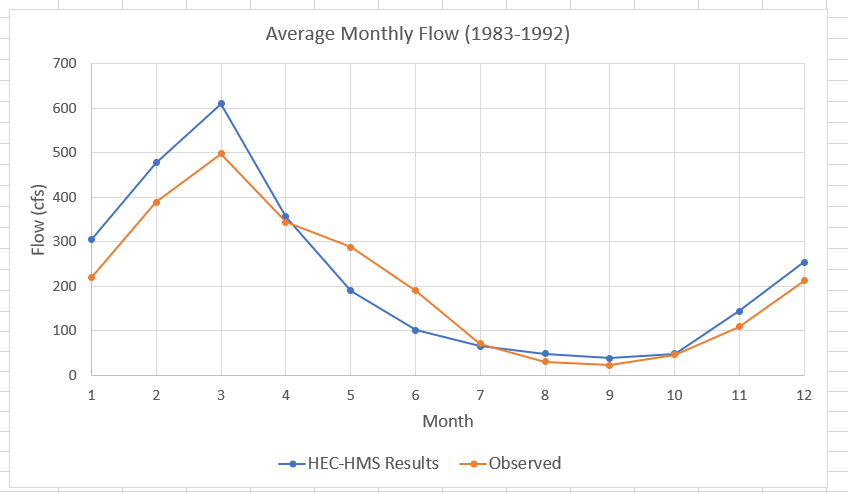
- The following figure shows the monthly average Flow results. You can see the outcome of incorrectly modeling SWE in December - March, instead of a portion of the precipitation being stored as snow, it is running off and the simulated Flow results are higher than observed for the December - March period.
- The following figure shows the monthly average SWE results. Notice that the results from HEC-HMS are much lower that the observed SWE for this time period. Before adjusting Loss and Baseflow parameter you should adjust the temperature index PX and Base temperatures to improve the modeled SWE results.
Adjust Model Parameter to Improve Performance
Calibration Tip
Recall that the PX Temperature is used to discriminate between precipitation falling as rain or snow. Increasing the PX Temperature will cause more precipitation to fall as snow, resulting in a deeper snowpack.
When the air temperature is higher than the Base Temperature, snowmelt occurs. Increasing the Base Temperature will cause the snowpack to last longer since higher temperatures are required to melt the snow.
For linear baseflow, the number of routing steps can be used to subdivide the routing through each layer and is related to the amount of attenuation during the routing. Minimum attenuation is achieved when only one routing step is selected. Attenuation of baseflow increases as the number of steps increases. Increasing the GW 1 and GW 2 Coefficients will shift the baseflow hydrograph later in time. Conversely, decreasing these coefficients will shift the baseflow hydrograph sooner in time.
- Start by adjusting the PX and Base parameters to improve the simulated SWE results. You can look at results from HEC-HMS, and also follow the steps above to compute monthly SWE and update the spreadsheet.
- Your goal is to have a monthly NSE of 0.8 or better and a PBIAS less than +/- 10 percent.
- After you are satisfied with the model's performance in simulating SWE, start adjusting the constant loss rate and baseflow fraction parameters. Visually check that the Peak flows are similar to the observed peak flows; however, spend most of your time comparing monthly average flows.
- Your goal is to have a monthly NSE of 0.7 or better and a PBIAS less than 10 percent.
Download final project files here
Continue to Task 3. Validate the Model for Water Years 1993-2002