Download PDF
Download page Task 4. Perform a Period of Record Simulation for Water Years 1916-2018.
Task 4. Perform a Period of Record Simulation for Water Years 1916-2018
Return to Task 3. Validate the Model for Water Years 1993-2002
Last Modified: 2024-06-28 12:52:27.745
This tutorial demonstrates a process to validate an HEC-HMS model for a long term simulation by evaluating flow-frequency results.
Software Version
HEC-HMS version 4.12 was used to create this example. You can open the example HEC-HMS project with HEC-HMS v4.12 or a newer version.
HEC-SSP version 2.3-beta.5 was used to create this example. You can open the example HEC-SSP project with HEC-SSP 2.3 or a newer version. You can download HEC-SSP here: https://www.hec.usace.army.mil/software/hec-ssp/download.aspx.

Allotted Time
This task should take approximately 30 - 45 minutes to complete.
Introduction
Your goal in task 4 is to validate the model you developed in task 2 using a period of record simulation window and comparing simulated flow-frequency results to a flow-frequency curve developed using observed data. You can continue using the model you developed in task 2 or start with the model provided above.
Run the Period of Record Window
- Create a simulation run named POR. Select the TuleRiver_Cal basin model, Livneh meteorologic model, and the Period of Record control specifications. The time window for the period of record simulation is 01 January 1915 through 01 October 2018. For the flow frequency analysis, the 1915 water year will be ignored since we do not have data for the complete water year. We will have 103 years of simulated peak flows for the flow-frequency analysis.
- Run the simulation. The simulation should take about 8 minutes to complete.
- Look at the simulated and observed SWE results for the MF_TuleR_S20 subbasin. Does the calibrated model perform well during the period of record simulation? What do you notice about the simulated SWE throughout the entire period of record?
- Zoom into the 1967 water year. You can also open the time-series table for the MF_TuleR_S20 subbasin. See the figure below. The SWE increases over 20 inches in December. The total precipitation for the period December 4 through 7 is over 33 inches for the MF_TuleR_S20 subbasin.
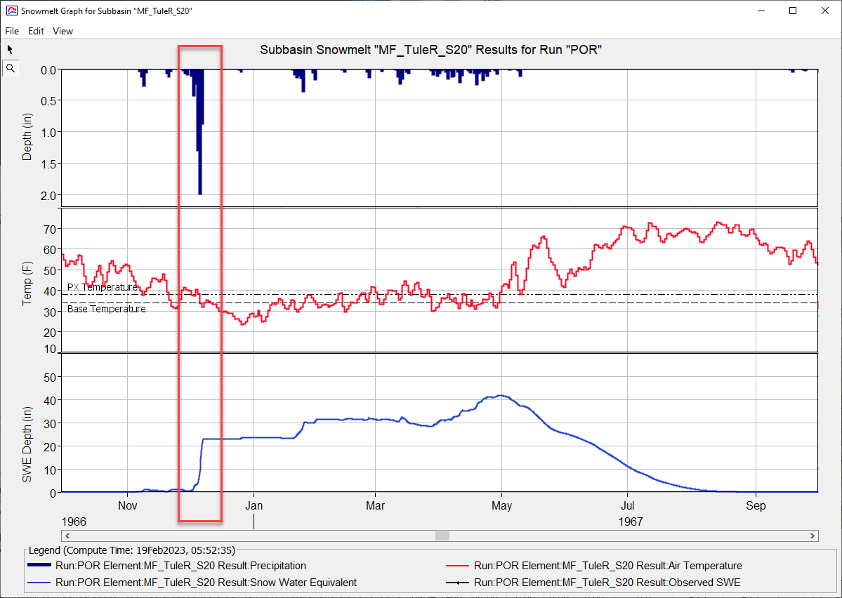
- Zoom into the 1967 water year. You can also open the time-series table for the MF_TuleR_S20 subbasin. See the figure below. The SWE increases over 20 inches in December. The total precipitation for the period December 4 through 7 is over 33 inches for the MF_TuleR_S20 subbasin.
- Look at the simulated and observed flow for the ReservoirInflow sink element. Does the calibrated model perform well during the period of record simulation? What do you notice about the simulated flow throughout the entire period of record?
- As shown in the figure below, there are a couple of patterns that stand out when looking at the simulated reservoir inflow. 1915 through 1931 seems to be dry period in the period of record. You could extract the precipitation time-series to verify. This could be an artifact of how the precipitation dataset was created or a drought period in the Western U.S. The largest floods of record occurred in the 1950s and 1960s. As shown in the SWE plot above, the excessive precipitation in December 1966 generated the flood of record shown below. The reservoir regulation manual contains information about the 1966 flood, the estimated peak discharge was 76,900 cfs and the peak 1-day flow was 40,000 cfs.
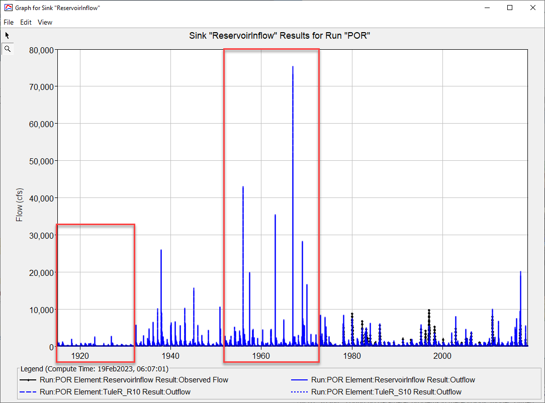
- As shown in the figure below, there are a couple of patterns that stand out when looking at the simulated reservoir inflow. 1915 through 1931 seems to be dry period in the period of record. You could extract the precipitation time-series to verify. This could be an artifact of how the precipitation dataset was created or a drought period in the Western U.S. The largest floods of record occurred in the 1950s and 1960s. As shown in the SWE plot above, the excessive precipitation in December 1966 generated the flood of record shown below. The reservoir regulation manual contains information about the 1966 flood, the estimated peak discharge was 76,900 cfs and the peak 1-day flow was 40,000 cfs.
- Follow the same steps contain in task 3 and compute the daily average flow for the ReservoirInflow sink element using HEC-DSSVue. Make sure you do this for results in the Period of Record simulation.
Evaluate Flow-Frequency using HEC-SSP
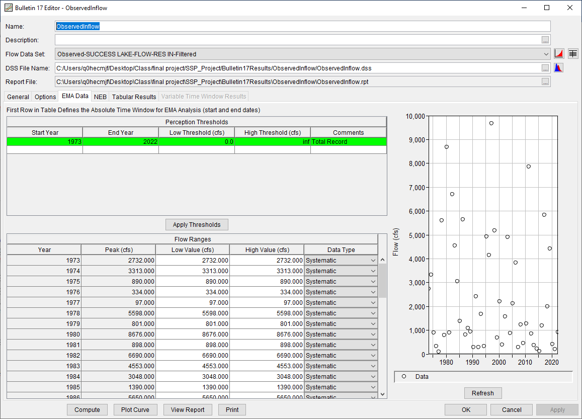
- Open the HEC-SSP project. You should notice observed daily average inflow has been added to the project and an Bulletin 17 analysis has been created and computed. You can refer to HEC-SSP manual to learn more about Bulletin 17 analyses.
- Open the ObservedInflow analysis and select the EMA Data tab. The period of record for observed inflow is 1973 - 2022.
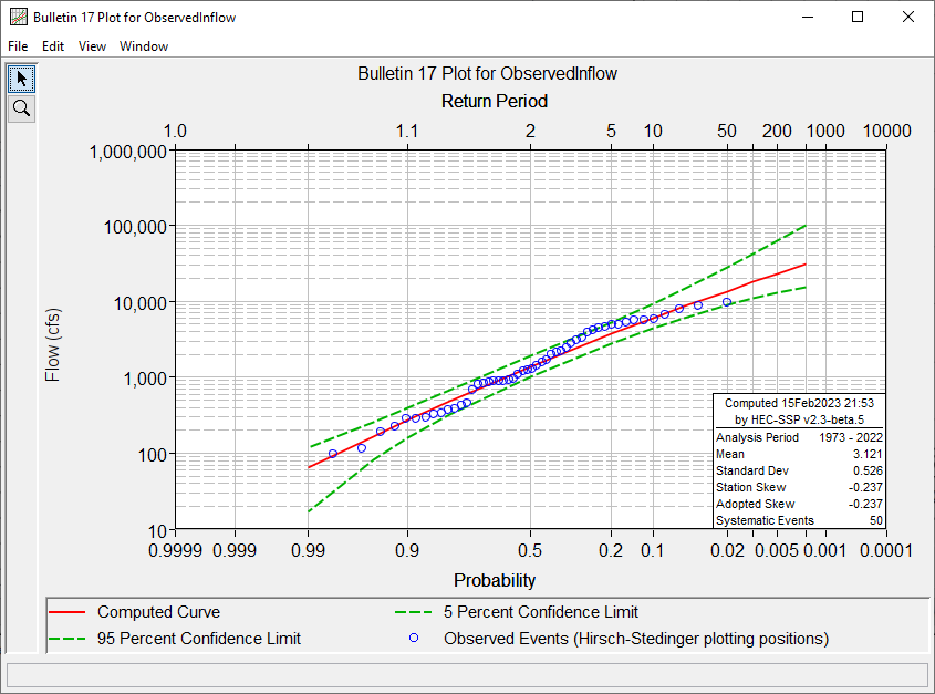
- Press the Compute button and then press the Plot Curve button to view the compute flow-frequency curve.
- Open the ObservedInflow analysis and select the EMA Data tab. The period of record for observed inflow is 1973 - 2022.
- Import the computed daily average flow dataset into the HEC-SSP project.
- Select Data | New | Traditional Import.
- As shown in the figure below:
- Enter a name of HEC-HMS Results.
- Choose the POR.dss file.
- Select the ReservoirInflow option for the Part B pathname.
- Add the 1Day Flow time-series to the bottom pane by double left-clicking on the record.
- Click the Import to Study DSS File button.
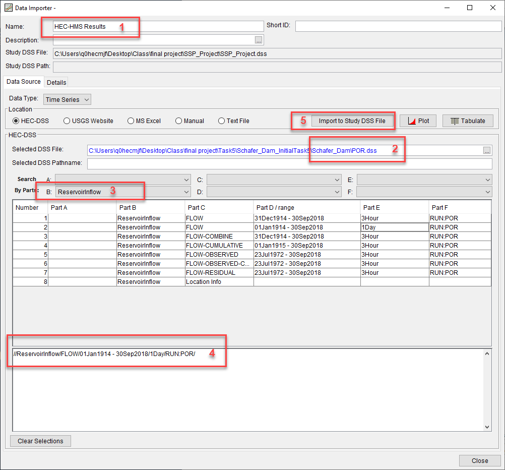
- You should see a new dataset, named HEC-HMS Results-ReservoirInflow-FLOW, added to the Data folder.
- Extract annual maximum daily average peak flows.
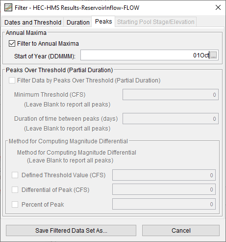
- Right Click on the daily average flow time series and choose Filter Data.
- As shown below, go to the Peaks tab. Check the box to Filter to Annual Maxima and then set the Start of Year to 01Oct.
- Click the Save Filtered Data Set As button. Then click OK in the Save as New Data Set window. The default name is fine.
- Right-click on the created annual maximum time series and select Plot. The following plot shows the annual maximum 1-day average flows from the HEC-HMS model simulation.

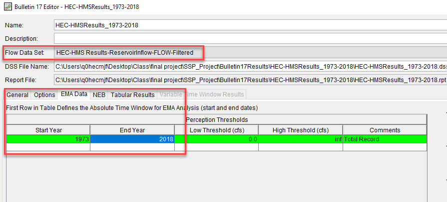
- Create a new Bulletin 17 analysis named HEC-HMSResults_1973-2018. As shown in the figure below, choose the HEC-HMS Results-ReservoirInflow-FLOW-Filtered peak flow dataset. Then go to the EMA Data tab and enter a start year of 1973 and end year of 2018.
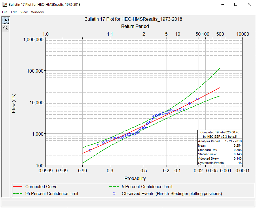
- Press the Compute button and plot the computed curve.
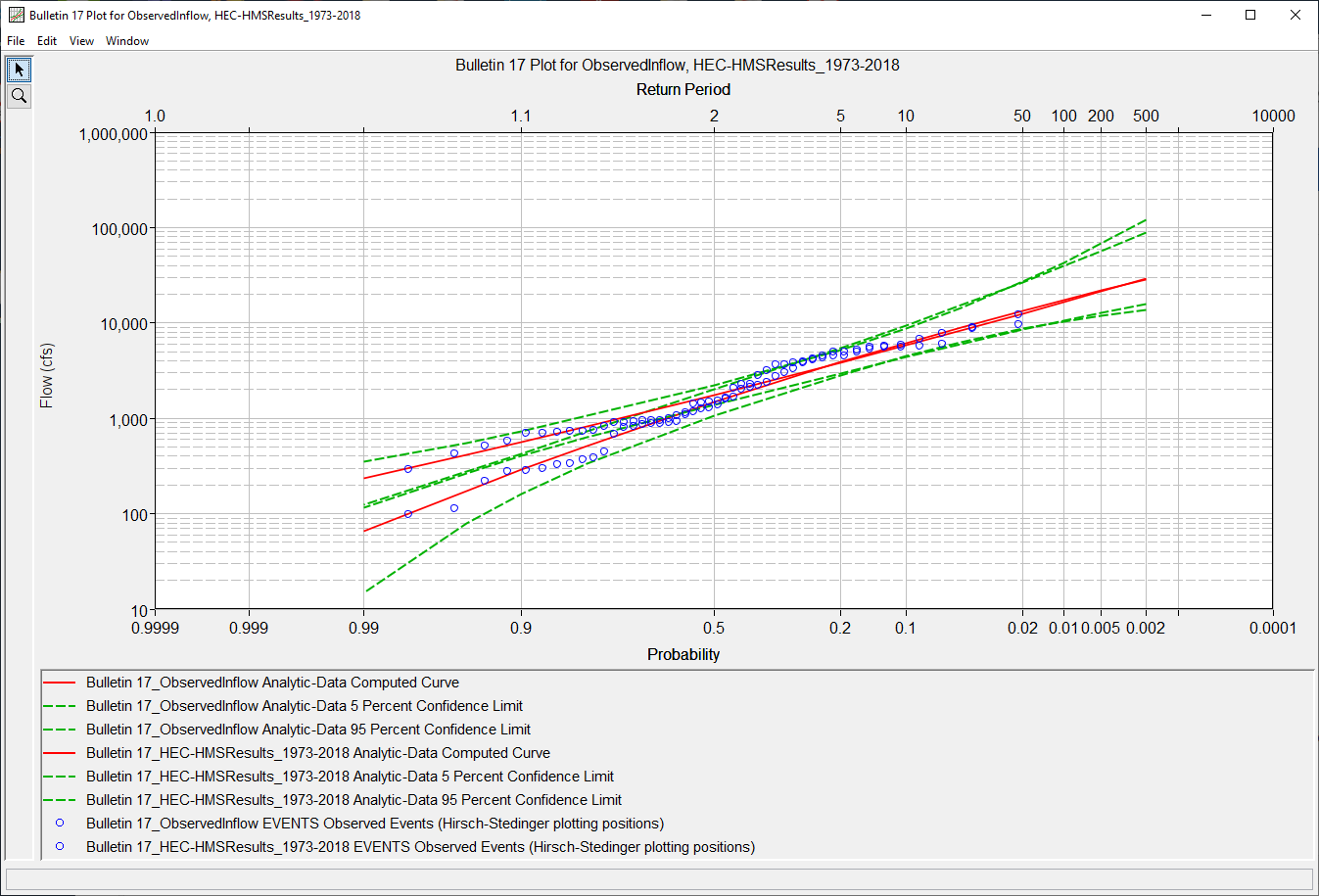
- Before comparing the observed data and HEC-HMS results 1-day average flow frequency curves, modify the End Year for the ObservedInflow Bulletin 17 analysis. Set the End Year to 2018 and click the compute button. This change will ensure we compare frequency curves using overlapping water years.
- You can compare the results from two Bulletin 17 Frequency analyses by selecting both in the study tree and then go to Results | Graph.
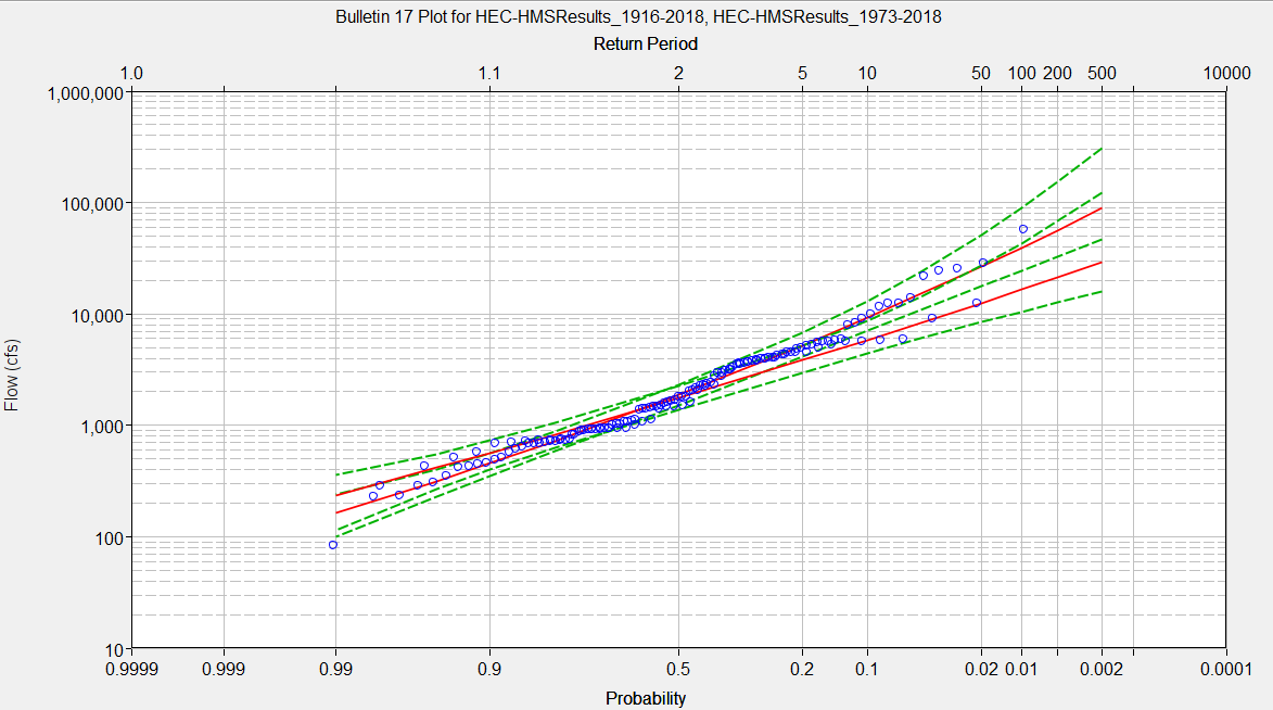
- Create a new Bulletin 17 analysis named HEC-HMSResults_1916-2018. As shown in the figure below, choose the HEC-HMS Results-ReservoirInflow-FLOW-Filtered peak flow dataset. Then go to the EMA Data tab and enter a start year of 1916 and end year of 2018.
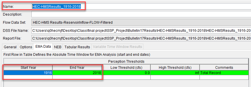
- Press the Compute button and plot the computed curve.

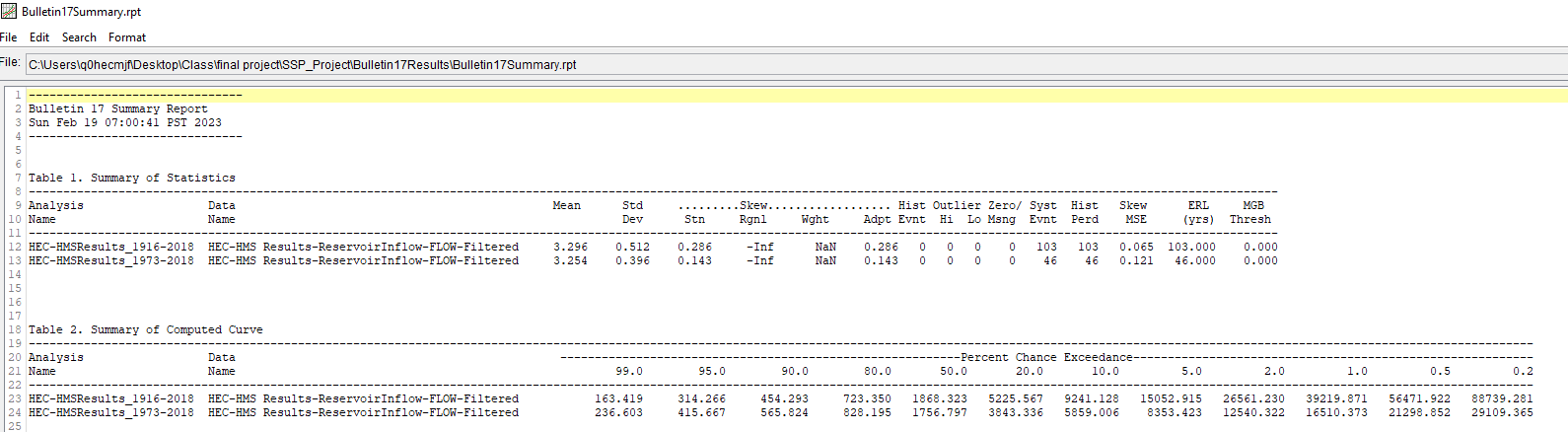
- Compare the short duration and long duration flow frequency curves.
Continue to Task 5. Document Final Parameters and Results