Last Modified: 2024-01-30 07:12:25.445

In this tutorial, you will create two types of time series data in HEC-HMS: precipitation gages and discharge gages.

Software Version

HEC-HMS version 4.12 beta 3 was used to create this example. You can open the example project with HEC-HMS 4.12 or a newer version.

Project Files

Download initial project files provided on the Shared Component Data Overview page

Step 1. Download and extract the HEC-HMS project .

• Open the project in HEC-HMS version 4.12 Beta 3 or later.

You will see that this project has a basin model already created for you. Expanding the basin model folder in the project tree, you should see the following components:

Creating a Precipitation Gage with HEC-DSS data

Precipitation gage data can be used as one type of boundary condition for hydrologic simulations. Frequently, gage data is used to model hydrology for time periods and locations where radar or multi-sensor precipitation estimates are not available. This example will show how to create a precipitation gage and link it to data contained in an HEC-DSS file, but any type of time-series data can be linked to an HEC-DSS file.

Step 2. Create a new precipitation gage time series

 Components menu | Create Component | Time-Series Data...

Step 3. A new window will appear that allows you to create a new time-series data. The default data type is for precipitation gages, but when you want to create other types of time-series data, make sure you change the data type before giving it a name and a description. You have been provided precipitation gage data for three stations near the Mahoning Creek watershed, and you will create a gage for the station nearest the city of Punxsutawney. It has a station ID of PNXP which you should enter as the time series data name. A description is optional but always a good idea. Provide a reasonable description for these data, and then select the Create button.

Step 4. You should notice that a new folder is added in the tree view for the Watershed Explorer on the left side for time-series data. Expand this folder to see that there is a folder for precipitation gages. HEC-HMS organizes Shared Data components by type, so multiple time-series data can have the same name as long as they are not of the same type. Expand the precipitation gages folder to see the PNXP gage, and then select the PNXP gage so that you can see its settings.

Step 5. Precipitation data for the PNXP gage has been provided in a DSS file in the project folder. In order to link this data to the new precipitation gage, select Single Record HEC-DSS from the Data Source option for the time-series gage.

Step 6. The options in the component editor will change so that you can select the precipitation data in the HEC-DSS file:

Step 7. The red asterisk indicates that these settings are required. First, browse to the provided HEC-DSS file by selecting the folder icon to the right of the DSS Filename text field. The DSS file is in the HEC-HMS project folder, in a subfolder called "data." The file is called "gage_precip.dss." Select this HEC-DSS file and press Select.

Step 8. This will populate the DSS Filename text field. The DSS Pathname (which specifies which data you want out of the HEC-DSS file) also needs to be populated. Select the button to the right of the DSS Pathname text field (it looks like a white rectangle with horizontal lines on it.) This will open a viewer for the HEC-DSS file.

Step 9. You are interested in the precipitation data for the PNXP gage, so select the row with the Part B that says PNXP (you could also filter for Part B in the search dropdown box). Then, press the Set Pathname button. This will populate the DSS Pathname text field. After specifying the DSS Filename and DSS Pathname, your component editor should look something like this:

Step 10. Save your project by clicking the save icon in the toolbar, or by pressing Ctrl+S. You should notice that the Units and Time Interval settings will automatically update to match the data in the HEC-DSS file.

Step 11. Next, you will specify the location of the precipitation gage by entering data in the remaining six text fields. The PNXP gage is located at 40°56'21"N, 79°00'31"W. HEC-HMS uses the convention that negative values of latitude are in the southern hemisphere, and negative values of longitude are used for the western hemisphere. Enter the correct values in the component editor, and then save your project.

40°56'21"N, 79°00'31"W is equivalent to 40.93917°, -79.0086°.

NOTE: If you don't see minutes and seconds option, change settings for Latitude and Longitude in Tools | Program Settings.

Why is the location information important for a precipitation gage? What kinds of applications can you see that would require this?

Step 12. Finally, you will create a time window for the precipitation gage. Time windows are only used to view sub-sets of the precipitation gage data and do not affect hydrologic simulation. They are optional. The default time window of 01Jan2000 00:00 - 02Jan2000 00:00 does not contain any of the observations contained in this precipitation data. The first event contained in this gage data is from 01Apr1994 00:00 - 30Apr1994 24:00. Right-click on the PNXP precipitation gage in the Watershed Explorer and select Create Time Window.

Step 13. Enter the correct start and end date and time in the new window, and press Add, and then press Close.

Step 14. You should notice a new time window underneath the PNXP gage in the watershed explorer. Click on this time window so that you can view the precipitation data as a graph.

Step 15. Delete the default time window (01Jan2000 - 02Jan2000) by right clicking on it and selecting Delete Time Window.

Creating a Discharge Gage with Manual Entry Data

Discharge gage data can be used to compare the results of simulations for a historic event to the actual streamflow that occurred. This is an important part of the model calibration process. This example will show how to populate a discharge gage with manually-entered data, but any type of time-series data can be entered in such a way.

Step 16. Create a new discharge gage time series  as follows:

 Components menu | Create Component  | Time-Series Data...

Step 17. A new window will appear that allows you to create a new time-series data. The default data type is for precipitation gages, and you will want to change the data type before giving it a name and a description. You have been provided stream gage data for the discharge gage on Mahoning Creek at Punxsutawney, and you will create a discharge gage for this station. It has a station ID of USGS 03034000 which you should enter as the time series data name. A description is optional but always a good idea. Provide a reasonable description for these data, and then select the Create button.

Step 18. Make sure the time-series data folder is expanded to see that there is a folder for discharge gages. Expand the discharge gages folder to see the USGS 03034000 gage, and then select it so that you can see its settings.

Step 19. You will be entering the observed discharge data from a provided Microsoft Excel spreadsheet that contains the half-hourly flow observations for the April 1994 flood event. The units are in cubic feet per second. Change the setting for units to the correct units, and then change the time interval to 30 minutes.

Step 20. Next, save your project by selecting the save icon in the toolbar, or by pressing Ctrl+S.

Step 21. Create a time window by right clicking on the USGS 03034000 discharge gage and selecting Create Time Window.

Step 22. Enter a start date and time of 01Apr1994 00:00 and an end date and time of 01May1994 23:30. Then, press Add, and then press Close.

Step 23. Delete the default time window (01Jan2000 - 02Jan2000) by right clicking on it and selecting Delete Time Window.

NOTE: You could also edit an existing time window by clicking on it and entering the new times.

Step 24. Select the time window you just created beneath the USGS 03034000 gage data. Click on the Table tab in the Component Editor. You will see a spreadsheet-like table that has the date-time pre-populated for the time window in the first column, and a column of blank entries to enter discharge data.

Step 25. In the HEC-HMS project folder, there is a sub-folder called data and it contains a spreadsheet called USGS03034000_Apr1994.xlsx. Navigate to that folder and open the spreadsheet in Microsoft Excel.

The spreadsheet has two columns of data. The first contains the same dates as were shown in the time series editor in HEC-HMS. The second column contains the data that you will want to copy into the empty fields in the time series editor of HEC-HMS.

Step 26. Select the entire column of discharge data beginning with the first 968 value (use ctrl + shift + Down Arrow to quickly select all of the data), and copy it from the spreadsheet. Then go back to HEC-HMS where the time series editor is open for the discharge gage. Right-click on the first cell of the editor and select Paste.

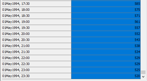
Step 27. The column will then be populated with the values from the spreadsheet. Scroll to the bottom to check to make sure that the last data value coincides with the last time value.

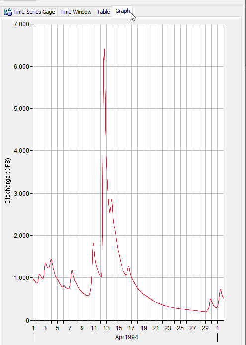
Step 28. Save your HEC-HMS project. You can view the graph of this discharge gage by switching from the Table to the Graph tab.

Step 29. Finally, you can verify that this discharge gage is now available to be added as observed flow in the basin model. Select the Sep2018 basin model and click on the MahoningCk subbasin element in the tree.

Step 30. In the Component Editor, switch to the Options tab. You will see that the menu item for Observed Flow is expandable, and that you can select the USGS 03034000 discharge gage. Only discharge time-series data are able to be selected in this menu. 

Project Files

Final project files provided on the Shared Component Data Overview page

Continue to Creating Paired Data