Download PDF
Download page Outflow Curve Option for an HEC-HMS Reservoir Element.
Outflow Curve Option for an HEC-HMS Reservoir Element
Software Version
HEC-HMS version 4.12 beta 5 was used to create this example. You can open the example project with HEC-HMS 4.12 beta 5 or a newer version.

Overview
The reservoir routing model requires information about the reservoir, such as the elevation-storage relationship, and information about physical structures, like spillways and other outlets. These regulating outlets are commonly simplified through use of a stage-storage-discharge relationship. Reservoir routing in HEC-HMS is based on a hydrologic routing method, which is concentrated on the concept of storage for the flood water.
In this tutorial you will add a reservoir element to a basin model and configure the reservoir element and develop storage-discharge relationships to use the Outflow Curve routing method. We will compare simulated and observed reservoir elevation to evaluate the performance of the calibrated outflow curve. Observed discharge from the reservoir has already been added to the project along with some additional data needed to configure the reservoir element and run a simulation. As mentioned in Introduction to Modeling Reservoir Operations with HEC-HMS, the HEC-HMS model for the watershed upstream of the reservoir has been calibrated to the simulation time window used for this tutorial.
Regulated outlets
Regulated outlets controlled by gates are a common feature of flood control reservoirs. Varying gate settings mean that a single stage or storage value can be associated with different outflow magnitudes depending on operations on a given day. Many flood control dams are operated with consideration to downstream constraints and “rate of release” constraints. Consequently, it can be challenging to construct a simple stage-discharge relationship for outlet works. To more simply model gate operations in HEC-HMS, the modeler can rely on historic data to fit a relationship to a distribution of stage and accompanying discharges.
- Plot several years of observed daily or hourly stage versus regulated discharge to see if there is a distinguishable trend. In this example we'll use hourly stage and regulated outflow for Lake Schafer Dam and Reservoir from 1989 to 2023 downloaded from the CDEC. This has already been downloaded and placed into the Excel workbook named OutflowCurve_Data_Initial.xlsx. The plotted data show no observable trend, so additional processing in Excel will be needed.

2. Data should be sorted by elevation from lowest to highest stage. This step has been completed and the data has been filtered for zeros, no data values and erroneous observations. Some QC of the raw outflow and stage data of your dataset will likely be necessary. Next, average the outflow over 5 FT bands using the AVERAGEIFS function in Excel. Input the AVERAGEIFS function (as shown in the figure below) into cells H2:H19.

3. (This step has been completed and the plot will be populated automatically after Step 3). Next, the average discharge over the five foot bands are plotted against a representative stage (taken as the center of the elevation band). Create a plot with G2:G19 as your independent variable on the x-axis and H2:H19 as the dependent variable on the y-axis. In the figure below, a clear trend is visible and a trendline and equation can be fit to the relationship and a full table of outlet releases can be computed. Right click on the data and select Add Trendline... to the data, select Polynomial under Trendline Options add check Display Equation on chart.
4. Input the coefficients of your polynomial function into cells K2:K4 in the format ax2 +bx + c. The first few cells have been filled in in column M to ensure there are no negative values and the discharge values are monotonically increasing with elevation. This equation will now populate the Stage-Outlet Works Discharge shown in Table 1. Your values may vary slightly based on the precision of your coefficients.

Table 1. Computed stage and outlet works discharge relationship.
| Stage, FT | Outlet Works, CFS |
| 556 | 0 |
| 560 | 0 |
| 565 | 0 |
| 570 | 0 |
| 575 | 10 |
| 580 | 18 |
| 585 | 22 |
| 590 | 32 |
| 595 | 47 |
| 600 | 69 |
| 620 | 215 |
| 640 | 454 |
| 652.5 (Spillway Crest) | 652 |
| 655 | 696 |
| 675 | 1,101 |
| 680 | 1,217 |
| 685 | 1,338 |
| 690 | 1,466 |
| 691.5 (Top of Dam) | 1,505 |
| 695 | 1,600 |
| 700 | 1,739 |
Spillway Outflow
Uncontrolled spillway flow may be provided in the Water Control Manual for the dam in the form of a table or a plotted rating curve. If the rating curve is not available in a table form, there are web-based digitizer tools that can convert the curve from the plot to a table of values.
In the case of Success Dam, the full-range of spillway discharges are estimated according to the weir equation, Q = CLH^\frac{3}{2}. Where C is the coefficient of discharge, L is the length of the spillway measured perpendicular to the direction of flow, and H is the relative height of water above the spillway invert. The coefficient of discharge is assumed to be 3.0, the length of the spillway is 200 feet and the spillway invert is 652.5 FT. These values have been computed on the Spillway tab of the Excel workbook.
Table 2. Computed stage and spillway discharge relationship.
| Stage, FT | Spillway Flow, CFS (C= 3.0) |
| 652.5 | 0 |
| 655 | 2,372 |
| 660 | 12,324 |
| 665 | 26,517 |
| 670 | 43,925 |
| 675 | 64,036 |
| 680 | 86,527 |
| 685 | 111,167 |
| 690 | 137,784 |
| 691.5 | 146,133 |
| 695 | 166,240 |
| 700 | 196,423 |
Calibrating Weir Coefficient to Extrapolate
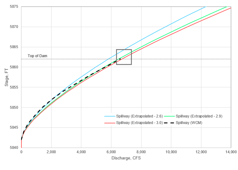
A weir equation should be used to extrapolate beyond the top of dam in lieu of linear extrapolation when possible. Spillway rating curves published in water control documents may not provide the weir equation or coefficient used to derive the values, in that case a simple calibration can be performed on the weir coefficient of discharge, C. Below, a range of C values were used to develop rating curves that were compared against the published rating curve for a different example dam. Because we're interested in high elevations, visually examine the behavior of the WCM rating curve at or near top of the dam. At the top of dam elevation in the example below, the WCM rating curve (black dashed line) is beginning to align more with a C value of 3.0. The final spillway rating curve for HMS routing should use published values below top of dam and be extrapolated beyond the top of dam with C= 3.0.
Dam Overtopping
To account for extreme events that may exceed the storage capacity of the dam, it's important that the stage discharge relationship is extended beyond the top of the dam. Rating curves for outlet works and spillways should be extrapolated beyond top of dam by three to five feet. Additionally, flow over the top of the dam must be estimated. The minimum measured crest elevation should be used as the invert of the dam top for the weir equation. The length of the dam top is 3,490 feet and the coefficient of discharge is assumed to be 3.0, and the minimum dam crest elevation is 691.5 FT. These values have been computed on the Dam Top tab of the Excel workbook.
Table 3. Computed stage and dam top discharge relationship.
| Stage, FT | Dam OT Flow, CFS |
| 691.5 | 0 |
| 692 | 3,702 |
| 695 | 68,557 |
| 700 | 259,463 |
Routing in HEC-HMS with Outflow Curve
All sources of outflow from the dam must be combined into a single curve to use the Outflow Curve method in HEC-HMS. The last column will be used for the discharge values in the Storage-Discharge table created in HEC-HMS.
Table 3. Computed stage and total discharge relationship for Schafer Dam.
| Stage, FT | Storage, AC-FT | Outlet Works, CFS | Spillway, CFS | Dam OT, CFS | Total Outflow, CFS |
| 550 | 0 | 0 | 0 | 0 | 0 |
| 556 | 49 | 0 | 0.0 | 0.0 | 0 |
| 575 | 2,558 | 10 | 0.0 | 0.0 | 10 |
| 580 | 3,838 | 18 | 0.0 | 0.0 | 18 |
| 585 | 5,347 | 22 | 0.0 | 0.0 | 22 |
| 590 | 7,187 | 32 | 0.0 | 0.0 | 32 |
| 595 | 9,403 | 47 | 0.0 | 0.0 | 47 |
| 600 | 12,201 | 69 | 0.0 | 0.0 | 69 |
| 620 | 28,714 | 215 | 0.0 | 0.0 | 215 |
| 640 | 56,593 | 454 | 0.0 | 0.0 | 454 |
| 652.5 (Spillway Crest) | 82,886 | 652 | 0.0 | 0.0 | 652 |
| 655 | 90,712 | 696 | 2,372 | 0.0 | 3,068 |
| 675 | 157,337 | 1,101 | 64,036 | 0.0 | 65,137 |
| 680 | 177,382 | 1,217 | 86,527 | 0.0 | 87,744 |
| 685 | 198,574 | 1,338 | 111,167 | 0.0 | 112,505 |
| 690 | 220,883 | 1,466 | 137,784 | 0.0 | 139,250 |
| 691.5 (Top of Dam) | 227,222 | 1,505 | 146,133 | 0 | 147,638 |
| 692 | 234,000 | 1,519 | 148,952 | 3,702 | 154,173 |
| 695 | 254,022 | 1,600 | 166,240 | 68,557 | 236,397 |
| 700 | 287,392 | 1,739 | 196,423 | 259,463 | 457,625 |
- Open the HMS project ReservoirExample.hms. In the TuleRiver basin model, add a reservoir element to the project, named Schafer_Dam. Connect the ReservoirInflow junction to the new reservoir element.
- Create a new Storage-Discharge table with the Paired Data Manager and name it Store-Discharge. Copy in the storage and total outflow values from Combined Curve tab of the Excel sheet in the appropriate columns in HMS.
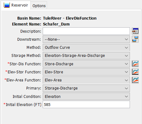
- Expand the basin model and Select the Schafer_Dam element. Edit the Reservoir Component Editor to use Outflow Curves as the routing method.
- Set the Storage Method to Elevation-Storage-Area-Discharge. Set each of the paired functions as shown below. Storage-Discharge should be the primary curve and the Initial Condition should be set to elevation 585.0 FT.
5. Open the Options tab for the Schafer_Dam reservoir element. As shown below, choose the Reservoir_Outflow gage for Observed Outflow and the Reservoir_Elevation gage for Observed Pool Elevation.
6. Run the simulation WY2017-2018-Outflow Curve and view the results graph of the Schafer Dam reservoir element.
Results Discussion
Examine the model performance of reservoir routing against the observed reservoir elevation using the outflow curve routing method. Next, refer to the results of the Rule-Based Option for an HEC-HMS Reservoir Element and compare model performance between the two routing methods.
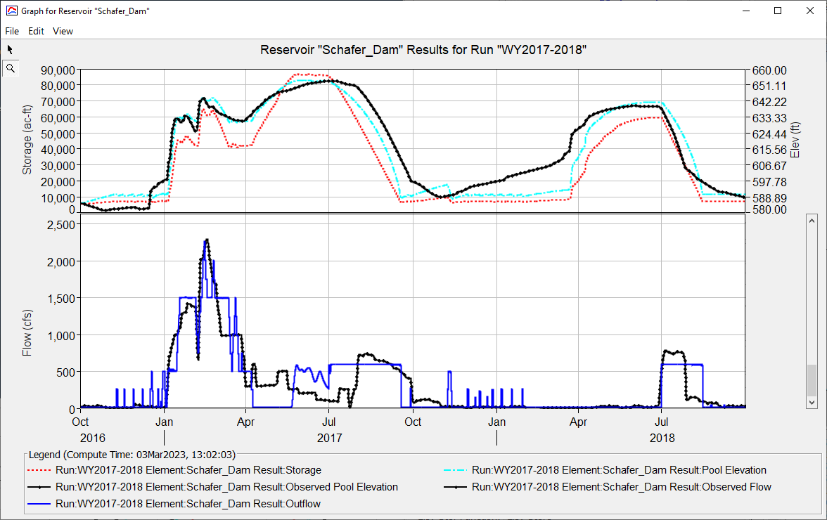
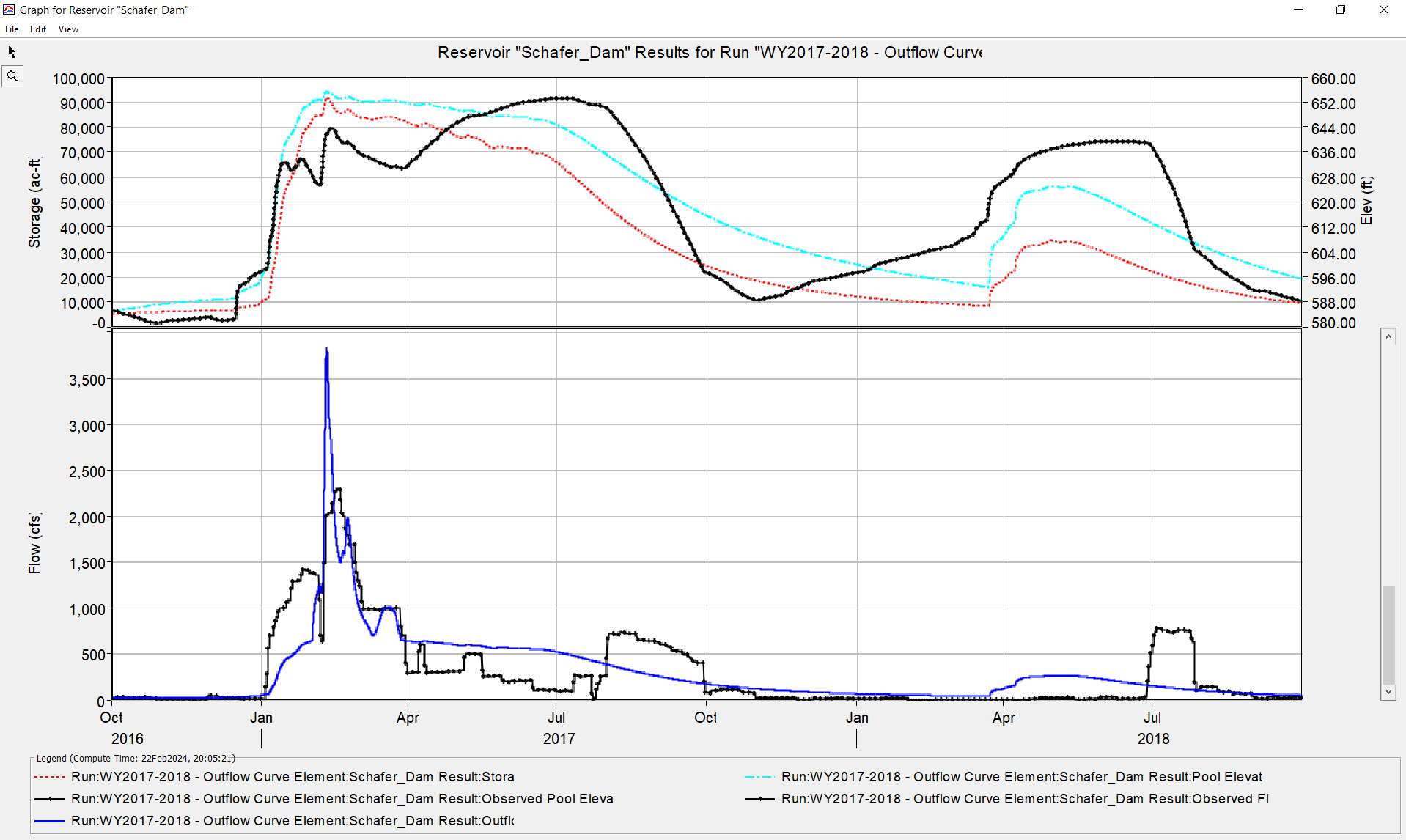
The model performance with respect to reservoir elevation/storage is better when the reservoir is routed with rule-based operations (top) as compared to outflow curve routing (bottom). Complex rules and operating guidelines are not easily captured in a single outflow curve and for most daily operations and routing of non-extreme events outlet works operations are crucial for accurately modeling outflow.
Question
- When might a single outflow curve would be a more appropriate routing method?
The Outflow Curve routing method is ideal when a reservoir doesn't have a complex release schedule or when modeling large inflow events during which the discharge through is negligible in comparison with total discharge from the dam. In the case of Success Dam, when the pool is near the top of dam, the estimated releases from the outlet works account for around 1% of total outflow. This routing method would be well suited for modeling a Probable Maximum Flood through a reservoir.