Download PDF
Download page Evaluating Temperature Index Snowmelt Parameter Sensitivity (Event Simulation).
Evaluating Temperature Index Snowmelt Parameter Sensitivity (Event Simulation)
Last Modified: 2023-07-13 10:41:15.252
Software Version
HEC-HMS version 4.11 was used to create this example. You can open the example project with HEC-HMS v4.11 or a newer version.

Introduction
The Temperature Index (TI) snowmelt method was the first snowmelt method included in HEC-HMS. Information on the Temperature Index snowmelt method can be found in the HEC-HMS User's Manual and the HEC-HMS Technical Reference Manual.
The following parameters are required to use this method:
- PX Temperature
- Base Temperature
- ATI-Coldrate Coefficient
- Dry Melt Rate
- Rain Rate Limit
- Wet Melt Rate
- Cold Limit
- Ground Melt Rate
- Liquid Water Capacity
In this tutorial, a parameter sensitivity analysis will be performed using the Uncertainy Analysis compute option in HEC-HMS and a regression analysis in Microsoft Excel. In evaluating parameter sensitivity, we are trying to answer the following questions:
- Which parameters play the largest role in the outputs of interest?
- Which parameter should be investigated (and uncertainty reduced) in future efforts?
This tutorial will evaluate Temperature Index snowmelt parameter sensitivity in an event simulation.
The following tutorial evaluates Temperature Index snowmelt parameter sensitivity in a continuous simulation, spanning a water year: Evaluating Temperature Index Snowmelt Parameter Sensitivity (Continuous Simulation)Study Area
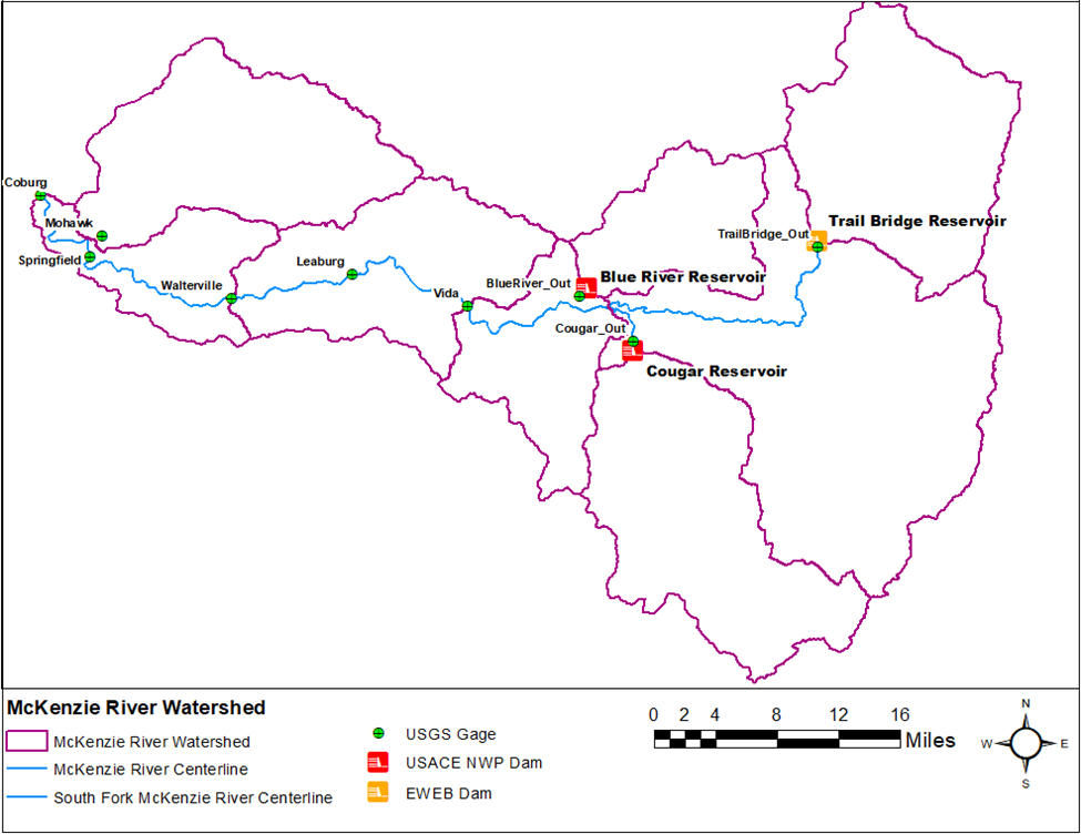
The McKenzie River watershed is located in western Oregon. The 90-mile river is a tributary of the Willamette River, which ultimately flows into the Columbia River north of downtown Portland. The McKenzie River watershed encompasses a drainage area of approximately 1,330 square miles. The headwaters of the McKenzie River are in the Cascade Mountains. The river flows south then west, through the communities of Finn Rock, Nimrod, Vida and Leaburg, before joining the Willamette River north of Eugene. Elevations in the McKenzie River watershed range from over 10,000 feet in the headwaters in the Cascades to approximately 300 ft near the confluence with the Willamette River. There are seven major dams in the McKenzie River watershed, two owned and operated by USACE Portland District (NWP) and five owned and operated by the Eugene Water and Electric Board (EWEB).
Review Existing HEC-HMS Project
An HEC-HMS project named McKenzie has already been created for you. This HEC-HMS project contains a Basin Model named Dec_2011_Feb_2012, a Control Specification named Dec2011-Feb2012, several Time Series, several Grid Sets, and a Terrain. As shown below, there is one subbasin element named SFMcKenzieRv_S10 which is connected to a junction element named Cougar_In representing inflow to Cougar Reservoir. The reservoir element Cougar_Res is connected to a junction element named Cougar_Out representing outflow from Cougar Reservoir. Cougar Reservoir is modeled using the Specified Release method. Observed time series, representing inflow to and outflow from Cougar Reservoir, are linked to the Cougar_In and Cougar_Out junctions, respectively. The subbasin was originally delineated using terrain data downloaded from the USGS National Map Viewer.
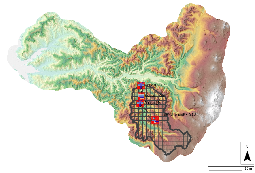
The subbasin element was configured to use a 2000-meter SHG Structured discretization, the Simple canopy method, the Deficit and Constant loss method, the ModClark unit hydrograph transform method, and the Linear Reservoir baseflow method. The previously-mentioned observed SWE and discharge time series were linked to the subbasin and junction elements as observed time series, respectively.
Data
The time period spanning 14Dec2011 through 12Feb2012 will be simulated within this tutorial using a 1-hour time step. The following data has been collected and imported to the existing HEC-HMS project for your use:
| Data Type | Source |
|---|---|
| Precipitation | Analysis of Record for Calibration (AORC) and Parameter-elevation Regressions on Independent Slopes Model (PRISM) |
| Air Temperature | Analysis of Record for Calibration (AORC) |
| Snow Water Equivalent Depth | Subbasin-Averaged Time Series from Snow Data Assimilation System (SNODAS) data |
Create a New Meteorologic Model and Parameterize
Before performing a parameter sensitivity analysis, a meteorologic model must be created. Boundary conditions that are required to use the Temperature Index snowmelt method include:
- Precipitation
- Air Temperature
- Download the McKenzie_Start project and unzip the file.
- Start HEC-HMS (version 4.11 or newer) and open the McKenzie project.
- Expand the Basin Model folder in the Watershed Explorer and select the Dec_2011_Feb_2012 basin model. Notice that the basin model contains a single subbasin named SASP.
- Create a Meteorologic Model by selecting Components | Meteorologic Model Manager. Click the New... button. Name the meteorologic model Dec2011-Feb2012 and click the Create button.
- Close the Meteorologic Model Manager window.
- Expand the Meteorologic Model folder in the Watershed Explorer and select the InSitu meteorologic model.
- From the Component Editor, select the following:
- Unit System: U.S. Customary
- Shortwave: --None--
- Longwave: --None--
- Precipitation: Gridded Precipitation
- Temperature: Gridded Temperature
- Windspeed: --None--
- Pressure: --None--
- Dew Point: --None--
- Evapotranspiration: Gridded Hamon
Replace Missing: Set To Default
The Meteorologic Model Component Editor should appear as in the figure below.
- Select the Gridded Precipitation node from the Watershed Explorer. Select Dec2011-Feb2012_AORC_PRISM from the Grid Name drop-down menu.
- Select the Gridded Temperature node from the Watershed Explorer. Select Dec2011-Feb2012_AORC from the Grid Name drop-down menu.
- Select the Gridded Hamon node and make sure that the Hamon Coefficient is set to 0.0065 (default value).
- Save the project.
Create and Compute a Simulation Run
- Create a Simulation Run by selecting Compute | Create Compute | Simulation Run.... Name the run Dec_2011_Feb_2012 and select the Next button. Select the Dec_2011_Feb_2012 basin model, the Dec2011-Feb2012 meteorologic model, and the Dec2011-Feb2012 control specifications on the following screens. Select the Finish button.
- Select the Dec_2011_Feb_2012 simulation from the Compute Selection Box in the Toolbar.
- Click the Compute button
 to run the simulation.
 - Navigate to the Results tab and expand the Simulation Runs folder.
- Select the Dec_2011_Feb_2012 simulation and expand the SFMcKenzieRv_S10 subbasin, Cougar_In junction, and Cougar_Res reservoir.
- Hold the keyboard Ctrl button and select the following time series:
- SFMcKenzieRv_S10: Observed SWE and Snow Water Equivalent
- Cougar_In: Outflow and Observed Flow
- Cougar_Res: Pool Elevation and Observed Pool Elevation
- Select the Plot button
 from the Toolbar. The results should appear as in the figure below.

The Dry Melt Rate can be specified using (1) an Annual Pattern, (2) an ATI Function, or (3) a Fixed Value.

In this tutorial, the Dry Melt Rate was described using a Fixed Value. Currently, only constant parameters can be sampled within the Uncertainty Analysis. Annual Patterns and ATI Functions are not currently supported within an Uncertainty Analysis. However, the Temperature Index snowmelt method is typically parameterized using an ATI Function for the Dry Melt Rate.
The following tutorials contain options to calibrate the Temperature Index snowmelt method using an ATI Function for the Dry Melt Rate:
Create and Compute an Uncertainty Analysis
- Create an Uncertainty Analysis by selecting Compute | Create Compute | Uncertainty Analysis....
- Name the Uncertainty Analysis U_D2011_F2012 as shown in the figure below. Click the Next> button.

- Select the Dec_2011_Feb_2012 basin model. Click the Next> button.
- Select the Dec_2011_Feb_2012 meteorologic model. Click the Finish button.
- Navigate to the Compute tab. A few folder titled Uncertainty Analyses was created. Expand the folder and select the U_D2011_F2012 analysis.
- In the Component Editor, select the gear icon next to the Analysis Points field. Click the checkbox next to the Snow Water Equivalent and Pool Elevation time series as shown in the figure below.

- Click the Save and Close buttons.
- In the Component Editor, enter the following for the Start Date/Time and End Date/Time:
- Start Date: 14Dec2011
- Start Time: 0000
- End Date: 12Feb2012
- End Time: 0000
- Select a Time Interval of 1 Hour from the drop-down menu.
- Enter 1000 in the Total Samples field. The Total Samples refers to the number of times the program will sample new parameter values and run a simulation.
- Right click on the uncertainty analysis and select Add Parameter.
- Repeat the above step 7 more times to add a total of 8 parameters.
For each parameter, select subbasin SFMcKenzieRv_S10 in the Element drop-down menu.
On the Parameter tab, select Simple Distribution from the Method drop-down menu and Uniform from the Distribution drop-down menu. The uniform distribution was used for this parameter sensitivity analysis because no information about parameter distributions was available.
Enter the Minimum and Maximum for each parameter using the values in the table below. For the uniform distribution, the Minimum and Lower values are the same and the Maximum and Upper values are the same. Do not enter the units in HEC-HMS; they are provided for clarity. The Parameter tab for Cold Limit is shown in the figure below.
The Ground Melt Rate parameter describes snow melt that results from the transfer of heat from the ground beneath the snowpack. This parameter was not included in the Uncertainty Analysis because it is almost always set to 0 in/day.
The ATI-Coldrate Function was not sampled in the Uncertainty Analysis. However, this parameter has a significant impact on the simulation results and should be calibrated.
Parameter
Distribution
Minimum
Maximum
Units
ATI-Coldrate Coefficient
Uniform
0.1
0.5
-
Base Temperature
Uniform
29 35 deg F PX Temperature
Uniform
29 35 deg F ATI-Meltrate Coefficient
Uniform
0.03 0.07 in/deg F-day Cold Limit
Uniform
0.01 0.5 in/day Liquid Water Capacity
Uniform
0 10 % Rain Rate Limit
Uniform
0 1 in/day Wet Melt Rate
Uniform
0 0.5 in/day 
Turn off notes and warnings in the Message Log by selecting Tools | Program Settings.... Navigate to the Messages tab. Under the Display messages in the message log and Write messages to the log file sections, uncheck the boxes next to Notes and Warnings, as shown in the figure below. Displaying and saving messages increases the run time of the Uncertainty Analysis.

Compute the Uncertainty Analysis.

The simulation will take approximately 25 minutes to compute.
Extract Sampled Parameter Values
- Navigate to the Results tab. Expand the Uncertainty Analyses folder and select the U_D2011_F2012 uncertainty analysis. The Results tab should resemble the figure below.

HEC-HMS provides the sampled parameter values for each realization. In addition, the reservoir pool elevation time series, maximum reservoir pool elevation, SWE time series, and maximum SWE value for each realization are provided. Select a Parameter node to view the sampled parameter values, as in the figure below.
- Open each Parameter node and copy the sampled parameter values to an Excel spreadsheet. Include a data label for each parameter (e.g. "PX Temperature").
- Expand the Cougar_Res reservoir node and select the Maximum Pool Elevation time series node. Copy the output to Excel. Include a data label for the maximum reservoir pool elevation output.
- Expand the SFMcKenzieRv_S10 subbasin node and select the Maximum SWE time series node. Copy the output to Excel. Include a data label for the maximum SWE output.
Perform a Multiple Linear Regression Analysis in Excel
The parameter values are generated through random sampling. Your parameter values will be different from the values shown in this section unless the same Seed Value is used in the HEC-HMS Uncertainty Analysis. The Seed Value is used to itialize the random number generator. In general, it is not advisable to change the Seed Value unless you are trying to duplicate results.
- Compute the mean and standard deviation of each parameter and the maximum SWE using Excel functions AVERAGE and STDEV.S. The Excel spreadsheet should look similar to the figure below.

Before performing a regression analysis, the sampled parameters and maximum SWE output must be standardized. The 8 parameters have different units and scales. Standardization is needed so that parameters with larger standard deviations do not have greater influence on the regression results. In addition, standardization ensures that the regression coefficients have uniform units. The parameters and output were standardized by subtracting the mean and dividing by the standard deviation:
Z_i = \frac{X_i - \bar{X}}{\hat{\sigma}} - The mean and standard deviation for each standardized variable should be 0 and 1, respectively. The results of the standardization should look similar to the figure below.

- Multiple linear regression can be performed in Excel using the Analysis ToolPak. Select File | Options. Navigate to the Add-ins tab on the left side of the Excel Options dialog box. On the bottom of the dialog box, select Excel Add-ins from the Manage drop-down menu and click the Go... button. Select the check box next to the Analysis Toolpack add-in, as in the figure below. Click the OK button to close the dialog box.

- Navigate to the Data tab | Analysis section | Data Analysis option.
- Select Regression in the Data Analysis dialog box. Click the OK button.
- In the Regression dialog box, make the following selections:
- The Input Y Range is the range of cells containing the maximum reservoir elevation data (including the data label).
- The Input X Range is the range of cells containing the standardized sampled parameters (including the data labels).
- Check the Labels box to indicate that data labels were included in the Y and X ranges.
- Under the Output Options, enter Results in the field next to New Worksheet Ply to save the regression analysis results in a new tab named Results.
- The Regression dialog box should resemble the figure below. Click the OK button perform the regression analysis.

Analyze Results
Navigate to the Results tab in Excel. The bottom table (boxed in red in the figure below) shows the results of the regression analysis. The coefficients are used to develop a linear regression of the general form:
y = ax + b
where a is the regression coefficient and b is the intercept. In this tutorial, 8 parameters were evaluated. Therefore, the linear regression takes the following form:
y = a_1x_1 + a_2x_2 + a_3x_3 + a_4x_4 + a_5x_5 + a_6x_6 + a_7x_7 + a_8x_8 + b
A negative regression coefficient means that smaller parameter values increase the maximum SWE and a positive regression coefficient means that larger parameter values increase the maximum SWE. The P-value indicates whether the dependent variable is statistically significant. Low P-values and high coefficient values indicate that the parameter has a significant impact on the dependent variable, or model output. 
- Select the 8 parameter labels and the corresponding regression coefficients.
Navigate to the Insert tab and select Recommended Charts in the Charts section. Select the Clustered Bar option. Click the OK button. The plot should look similar to the figure below.

The results of this parameter sensitivity analysis are specific to the South Fork McKenzie River watershed during the December 2011 - February 2012 event(s). The regression coefficients for Temperature Index snowmelt parameters will vary by location. A site-specific parameter sensitivity analysis should be performed for your modeling domain.
The PX Temperature and Base Temperature parameters have the largest negative regression coefficients. Recall that the PX Temperature is used to discriminate between precipitation falling as rain or snow. When the air temperature is higher than the Base Temperature, snowmelt occurs. Increasing the PX Temperature value causes more precipitation to fall as snow. Since the deeper snowpack did not completely melt during the event time period, the basin upstream of Cougar Reservoir produced less runoff. Increasing the Base Temperature causes the snowpack to last longer (i.e. produce less runoff during the event time window) since higher temperatures are required to melt the snow. The Wet Melt Rate has the largest positive regression coefficient. A large Wet Melt Rate value result in a high Maximum Pool Elevation value since more snow melts. Note that the Wet Melt Rate has a much larger impact on the Maximum Pool Elevation than the Dry Melt Rate during this event.
- Another way to evaluate model results is to compare individual model parameters to maximum pool elevation. Two parameters were selected for further analysis: Cold Limit and PX Temperature. The first plot is a comparison between the standardized Cold Limit and standardized Maximum Pool Elevation. The second plot is a comparison between the standardized PX Temperature and standardized Maximum Pool Elevation. The figures show that PX Temperature has a large impact on maximum pool elevation while Cold Limit has very little impact on maximum pool elevation.


Question: Repeat the regression analysis selecting Maximum SWE as the Input Y series. Create a tornado plot of the regression coefficients. Which parameter had the largest impact on the maximum SWE?

The relative magnitude of the regression coefficients is the same as the Maximum Pool Elevation analysis but the signs are reversed. Larger Base Temperature and PX Temperature values result in larger Maximum SWE values while a larger Wet Melt Rate results in smaller Maximum SWE values.
The regression coefficient magnitudes are different from the Maximum Pool Elevation values because parameters from modeling methods other than snowmelt (i.e. losses, transform, etc.) contribute to the watershed runoff.
The results of the regression analysis can inform calibration efforts. Modifying the Base Temperature, PX Temperature, and Wet Melt Rate will be most impactful when calibrating the model. The Excel spreadsheet used to perform the regression analysis is included below.