Download PDF
Download page Gridded Precipitation Method.
Gridded Precipitation Method
Return to Gage Weights Precipitation Method
Last Modified: 2024-07-26 16:56:40.135
Software Version
HEC-HMS version 4.12-beta.2 was used to create this example. You can open the example project with HEC-HMS 4.12-beta.2 or a newer version.

Introduction
In this tutorial, you will associate gridded precipitation data with a gridded precipitation method in a HEC-HMS Meteorologic Model. Gridded precipitation data comes from a number of sources. NEXRAD radar became operational in the 1990s across much of the United States and is the primary source of gridded precipitation data since then. Data available prior to the "radar era" are generally created by interpolating gage observations, reanalysis using numerical weather forecast or general circulation models, or a combination of both. Satellite observations began in the late 1980s and have improved in quality since, but are generally considered less reliable than other sources of precipitation observation. Modern products incorporate gage, radar, and satellite data into multi-sensor products with high spatial and temporal resolution, but such products have limited periods of record. A list of some gridded data sources commonly used in hydrologic modeling is located here: Gridded Data Sources.
You will model the September 2018 event in the Mahoning Creek watershed, and a HEC-HMS model containing the data you need in order to get started has been provided. The gridded precipitation data has already been imported and associated with a Grid Data component. For more information on importing grid data to your project see Creating Grid Data. The watershed has been represented using a single subbasin for the entire drainage area above the Punxsutawney gage.

Step 1. Begin by opening up HEC-HMS 4.12 or later. The project contains several elements in the Watershed Explorer, as below:

Step 2. Expand the Basin Models node of the Watershed Explorer tree and select the Sep2018 Basin Model. You will see that this model contains two elements, a Subbasin and a Sink. You should see in the Desktop map, a display that looks like the watershed above. There is a second Basin Model in this project, for the May 1996 event (which was used in the Gage Weights Precipitation Method tutorial). It is set up to work with the Gage Weights precipitation method.
What are two differences between the basin model for the May 1996 event, which is set up to work with gage weights, and the basin model for the September 2018 event, which is set up to work with gridded precipitation?
The MahoningCreek subbasin in the Sep2018 Basin Model contains a structured discretization method, and uses the ModClark transform method, instead of None and Clark for the May1996 model.
Step 3. Next, expand the Grid Data node of the tree and you will see that there are two types of grid data included in this model: precipitation and temperature. HEC-HMS keeps different types of grid data separate so that situations that call for a specific type of grid will only show that type of grid available. For this tutorial, the gridded precipitation method will only allow you to select precipitation grids as an input, for example.
Creating the Meteorologic Model
Step 4. Create a new Meteorologic Model by using the Components menu, then selecting Create Component > Meteorologic Model...
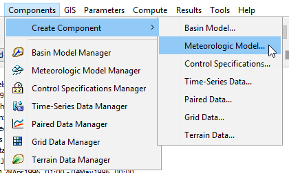
Step 5. For the name enter Sep 2018 Gridded. Descriptions are optional but generally good practice. Press Create to create the new met model.

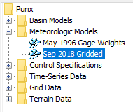
Step 6. Expand the Meteorologic Models node of the tree to see the Met Model you just created. Click on it to select it and so that you can edit it in the Component Editor.
Step 7. In the Component Editor, select the Gridded Precipitation method for precipitation. Make sure the Unit System is set to U.S. Customary.
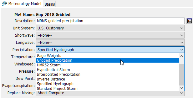
Step 8. You will see that an additional item appears beneath the Sep 2018 Gridded met model in the watershed explorer, an entry called Gridded Precipitation. Click on the Gridded Precipitation node to select it.

Step 9. After selecting the precipitation method, select the Gridded Precipitation node to open the Component Editor. For Grid Name, select the MRMS Precipitation grid component. The Time Shift (HR) option is used to transpose the grids in time so that differences such as time zone misalignment can be corrected.
It is good practice to handle time zone misalignment in data before importing the data to HEC-HMS. For example, all data should be converted to a common time zone, such as UTC or local time, and then saved to the project.
In this case, the observed discharge data and the precipitation data have been set up in the same time zone so no shift will be needed. Save your project.

Compare the parameterization of the gridded precipitation model and the gage weights model. What comparisons can you make between the gage weights method and the gridded precipitation method?
Gage weights takes point observations and uses a simple model in order to distribute them in space and time. However, it cannot create observations where there are no gages. Gridded data explicitly models the temporal and spatial variability of rainfall by providing an estimate for rainfall intensity everywhere. The gridded data method assumes that the gridded data are an accurate representation of the observed rainfall, and there are no parameters to adjust how the precipitation is applied to the watershed. The gage weights method allows some adjustment of its parameters to change how the combination of gage data estimates the basin-average precipitation, but relies on averaging a small number of point precipitation depth estimates.
Running a Simulation
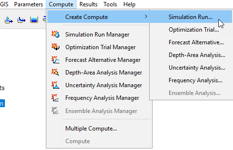
Step 10. Create a simulation run by choosing the Compute menu, then Create Compute > Simulation Run.... Name the simulation run September 2018, select the Sep2018 Basin Bodel, select the Sep 2018 Gridded Met Model, select the Sep2018 Control Specification, then press Finish.
Name the Simulation Run: Sep2018
Select Basin Model: Sep2018
Select Meteorologic Model: Sep 2018 Gridded
Select Control Specifications: Sep2018
Select Run2018 from drop down window and click the Compute All Elements button.

Add an Evapotranspiration Method to the Met Model
Optional Step 11. Add a Simple Canopy to the basin model so subbasin evapotranspiration can be calculated. Select the MahoningCreek subbasin in the Sep2018 Basin Model, and in the component editor choose Simple Canopy for the Canopy Method. The Canopy tab will be added to the Component Editor. Select the Canopy tab and set the Initial Storage (%) to 0, the Max Storage to 0.1, and the Uptake Method to Simple. Leave the default entries for Crop Coefficient and Evapotranspiration.

Step 12. Gridded temperature data have also been included in this model, so a gridded temperature-based evapotranspiration method can also be included in the Met Model. Select the Sep 2018 Gridded Met Model, and in the Component Editor set the Temperature method to Gridded Temperature and set the Evapotranspiration method to Gridded Hamon. Change the Met Model description so that it captures this update.

Step 13. Under the Sep 2018 Gridded Met Model there will now be additional nodes for Gridded Temperature and Gridded Hamon ET. Select the Gridded Temperature node so that it can be edited in the Component Editor.
What grid datasets are available to be selected in this menu? How many grid datasets are there in this HEC-HMS project?
Only one dataset is available, the RTMA dataset, which is a temperature grid set. There are two grid data in the HEC-HMS project, but the other is for precipitation data. It is important when creating grid data to select the correct data type, because HEC-HMS organizes grids so that the correct types are used in the correct places.
Step 14. Set the Temperature Grid to RTMA
Step 15. Select the Gridded Hamon node so that it can be viewed in the Component Editor, but leave the default value for the Hamon Coefficient. This value can be adjusted during the model calibration process, and is typically changed in continuous models.
Step 16. Re-compute the Sep 2018 simulation and view the results.
Continue to Creating an Inverse Distance Precipitation Model