Compute a Synthetic Unit Hydrograph for Several Historical Events

Now you will use synthetic unit hydrograph methods to reproduce the unit hydrographs for several historical events.

Synthetic unit hydrograph methods are generally preferred over the user-specified unit hydrograph method for several reasons including the following:

• Synthetic unit hydrographs can be easily used with different computational time steps.
  • No smoothing is required and the volume is guaranteed to be equal to one unit of runoff.
• Synthetic unit hydrograph methods allow users to efficiently and quantitatively peak the unit response, as required by USACE guidance.

HEC-HMS version 4.12-beta.5 was used to create this tutorial.  You will need to use HEC-HMS version 4.12, or newer, to open the project files.

Download the initial model files here:

PMF_Workshop_A_Initial.zip

Determine Clark Unit Hydrograph Parameters to Recreate the 1972 Unit Hydrograph

1. Open the PMF Workshop A HEC-HMS project.
2. The 1972 20-hour duration unit hydrograph, which was previously computed in Data Compilation, was entered as a time-series discharge gage.
   1. You can view this time series by navigating to Components | Create Component | Time-Series Data, clicking on the 1972 20-hour Unit Hydrograph, and clicking on the Table tab.
   2. The figure below shows the Graph tab for the unit hydrograph.
      
3. A basin model named 1972 Bald Eagle Calibration has been created for you.
   1. The 1972 Bald Eagle Calibration basin model contains one subbasin element name Bald Eagle Basin which represents the area upstream of Sayers Dam.
   2. This subbasin element has a drainage area of 338.6 square miles, the loss method has been set to "None", the transform method has been set to "Clark Unit Hydrograph", and the baseflow method has been set to "None", as shown in the following figure.
      
   3. Select the Transform tab.
      1. Set both the Time of Concentration (Tc) and Storage Coefficient (R) to 5 hours.
         
         

         These parameters can be estimated in numerous ways including regional regression equations and TR-55 methodology.  The Estimating Clark Unit Hydrograph Parameters tutorial contains steps that can be used to estimate these parameters.  As discussed in later steps, the Tc and R values will be adjusted so that the synthetic unit hydrograph matches the historic unit hydrograph.

4. Open the Options tab for the Bald Eagle Creek subbasin element and link the Observed Flow to the 1972 20-Hour Unit Hydrograph discharge gage. The computed unit hydrograph will be treated as observed flow and Tc and R will be adjusted manually to reproduce the unit hydrograph for the 1972 flood event.
5. A Precipitation Gage named 1-inch 20 hours has been created for you.
   1. The Units were set to "Incremental Inches" and the time interval was set to "1 Hour".
   2. The time window was set to be equivalent to the flow gage using a start date and time of 01Jan3000 00:00 and an end date and time of 07Jan3000 03:00.
   3. To recreate the unit hydrograph, one inch of precipitation must be distributed over the duration of the unit hydrograph. If 20 hours of excess precipitation generated the unit hydrograph for the 1972 event, then 1 inch of precipitation must be distributed over 20 hours. Therefore, 0.05 inches was entered for each hour starting at 01Jan3000, 01:00 and ending at hour 20:00 on 01Jan3000.
   4. The below figure shows the precipitation hyetograph with 0.05 inches distributed over 20 hours.
       
6. A Meteorologic Model named 1-inch Precip 20 hours was created for you.
   1. The replace missing option was set to "Set to Default" and the "Specified Hyetograph" was selected as the precipitation method.
   2. On the Basins tab, the Meteorologic Model was linked to the 1972 Bald Eagle Calibration basin model.
   3. Select the Specified Hyetograph node and note that the 1-inch 20 hours precipitation gage was chosen, as shown in the figure below.
7. A Control Specifications named Time Window has been created for you.
   1. Ensure the start date and time of 01Jan3000 00:00 and end date and time of 10Jan3000 00:00 has been entered.
   2. Note that a 1 Hour time interval has also been selected.
8. A Simulation Run named Calibrated 1972 Clark Model was created for you.
   1. The 1972 Bald Eagle Calibration basin model, 1-inch Precip 20 hours meteorologic model, and Time Window control specifications were selected when creating this Simulation Run. 
9. Run the Calibrated 1972 Clark Model simulation by clicking the Compute All Elements button .
   
10. Select the Bald Eagle Basin subbasin element and click the the Result Graph button,  , and the Summary Table button, .
    
    1. Leave the summary table and plot open so you can see results change as you modify the transform method parameters. The observed streamflow is represented by the black dotted line and the model's computed streamflow is represented by the solid blue line. 
11. As shown below, the initial Tc and R values (5 hours for both Tc and R) do a poor job recreating the unit hydrograph for the 1972 event.
     

12. Adjust the Tc and R parameters to reproduce the unit hydrograph for the 1972 flood event.

Question 1: What values of Tc and R did you find that adequately reproduced the 1972 unit hydrograph?

Question 2: What was the best Nash-Sutcliffe Efficiency (NSE) that was achieved during calibration?  For reference, the maximum possible NSE is 1.0.

Compare the 20-Hour and 1-Hour Unit Hydrographs for the 1972 Event

1. A Precipitation Gage named 1-inch 1 hour was created for you.
   1. The units were set to "Incremental Inches" and the time interval was set to "1 Hour".
   2. The time window should be equivalent to the flow gage:
      1. Start date and time = 01Jan3000 00:00
      2. End time/date = 07Jan3000 03:00.
   3. 1 inch of precipitation was entered for the first house and 0 was entered for the remaining time.
2. A Meteorologic Model named 1-inch Precip 1 hour has been created for you.  However, it will require slight modificatoins.
   1. Note that the replace missing option was set to "Set to Default" and "Specified Hyetograph" was selected as the precipitation method.
   2. On the Basins tab, ensure that the meteorologic model was linked to the 1972 Bald Eagle Calibration basin model.
   3. Select the Specified Hyetograph node and note that the 1-inch 1 hour precipitation gage was chosen for the Bald Eagle Basin.
3. Create a new Simulation named 1-inch 1 hour UH (1972).
   1. Select the 1972 Bald Eagle Calibration basin model, 1-inch Precip 1 hour meteorologic model, and Time Window control specifications.
4. Run the 1-inch 1 hour UH (1972) simulation by clicking the Compute All Elements button .
5. Compare the results from the 1-hour precipitation duration to the 20-hour precipitation duration to see how the unit hydrograph changes with respect to precipitation duration.
   1. Click on the Results tab, select the 1-inch 1 hour UH (1972) node, and click on the Bald Eagle Basin node.
   2. Click on the Results tab, select the Calibrated 1972 Clark Model node, and click on the Bald Eagle Basin node.
   3. Select the Bald Eagle Basin Outflow time series for both simulations to compare the results.  Note that when using the Clark unit hydrograph model, unlike a user-specified unit hydrograph, the unit hydrograph duration is automatically updated given the simulation time-step, as shown below.
      

The above figure compares the original 20-hour unit hydrograph (solid line) and the 1-hour unit hydrograph (dotted line). Both unit hydrographs have 1 unit of volume, as dictated by unit hydrograph theory. Converting the unit hydrograph from 20 hours to 1 hour increased the peak flow and shifted it forward in time. The graph was developed by holding down the Ctrl key and selecting the Outflow graph in the results of both simulations.

Determine the Most Conservative Unit Hydrograph

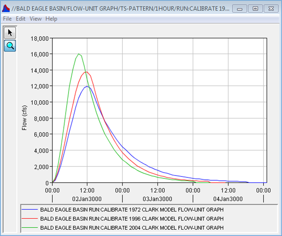
The figure below compares the 1-hour unit hydrographs that were determined for all three events (1972, 2004, and 1996). A separate HEC-HMS basin model was developed for each event and calibrated to the unit hydrographs using the Clark UH method. For a PA level PMF analysis, it is best to select the most conservative unit hydrograph for modeling. In general, the most conservative unit hydrograph is the one with the fastest timing and highest peak. Of the events considered, the 2004 unit hydrograph is the most conservative and will be used for the rest of this example. The Clark UH parameters for the 2004 event were Tc = 10 hours and R = 8 hours.

Question 3: Why do you think the 2004 event resulted in the most conservative unit hydrograph?

Continue to Apply a Peaking Factor to the Unit Hydrograph.