Last Modified: 2023-03-10 07:00:47.257

This workshop can be completed as part of the Workflows for Downloading, Importing and Manipulating Gridded Data or as a stand-alone activity.

HEC-HMS version 4.11-beta.10 was used to create this example. You can open the example project with HEC-HMS v4.11 or a newer version.

It is sometimes the case when modeling with gridded precipitation data that the data product that best captures the temporal distribution of rainfall does not best capture the cumulative volume of precipitation. The Normalizer Tool within HEC-HMS can be used to create a normalized precipitation grid that captures the temporal variability of one gridded dataset but the cumulative volume of another gridded dataset. For example, radar data collected at an hourly time step may adequately capture temporal variability over the simulation window, but a grid based on gage data collected at a daily time step may better capture the total volume of rainfall. For a detailed example showing how the Normalizer Tool computes the normalized grid, see the Normalizer User's Manual reference.

The two most important parameters the user must select when using the Normalizer Tool are the Normalization Period and Normalization Interval. The Normalization Period defines the time window that the normalized grids should be created for. The Normalization Interval defines the time window over which the volume of the source and normal grids are accumulated when computing the normalized grid. This tutorial demonstrates how altering the Normalization Interval changes the normalized grid and subsequent model results using a long-term, continuous HEC-HMS model of the Truckee River watershed. This tutorial does not describe how to use the Normalizer Tool. For a step-by-step tutorial describing how to use the Normalization Tool in HEC-HMS, see Correcting Precipitation Volume with the Normalizer Utility.

Optional:

You can practice obtaining one of the normalized data sets in this tutorial by normalizing raw MRMS rainfall grid with the raw gridded PRISM grid, provided with the Project Files. Follow the steps in the tutorial for Correcting Precipitation Volume with the Normalizer Utility.

Project files

Truckee_River_model.zip

Note that files are provided in a compressed folder and must be unzipped.

Open the Truckee River model

After unzipping the project files, open the Truckee River HEC-HMS model and navigate to the Results tab. Note there are five simulations that have already been computed. Each of the simulations span the entire 2017 water year (October 1, 2016 to September 30, 2017) and only differ by the gridded precipitation input. A description of each simulation is shown in the table below.

Simulations in the Truckee River HMS model

For each normalized grid, the Normalization Period began 10/1/2016 at time 1200 and ended 9/30/2017 at time 1200. 1200 was selected as the start and end time because the normal (PRISM) grids span time 1200 on day one through 1200 on day two.

Compare cumulative precipitation volumes

For each simulation in the model, select the subbasin element UpTruckeeRv_s10.

While holding the CTRL key, select "Cumulative Precipitation" in the "UpTruckeeRv_S10" results tree for the "WY2017_MRMS_raw" and "WY2017_PRISM_raw" simulations. Then, select the plot icon on HEC-HMS toolbar.


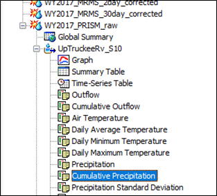
By the end of the simulation, the cumulative precipitation volume of the uncorrected hourly MRMS data (light blue line in the following figure) is much lower than the cumulative precipitation volume of the daily PRISM data (black line in the following figure).

Now, add the cumulative precipitation for the "UpTruckeeRv_S10" subbasin for the "WY2017_MRMS_1day_corrected" and "WY2017_MRMS_2day_corrected" simulations to the plot by holding the CTRL key, highlighting the "UpTruckeeRv_S10" cumulative precipitation result for all four simulations, and selecting the plot icon on the toolbar. The cumulative precipitation of the corrected, or "normalized", grids more closely matches the cumulative precipitation of the PRISM data.

Discussion question: Can you think of any reasons why the radar-based MRMS cumulative volume is significantly lower?

Zooming in to the plot during the Mar-Sep 2017 time period shows the normalized grids that used a Normalization Interval of 1 day resulted in a lower cumulative volume than the PRISM grids at the end of the simulation period. The normalized grids that used a Normalization Interval of 2 days had a higher cumulative precipitation volume, but the volume was still ultimately less than the PRISM data.

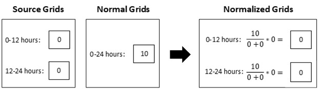
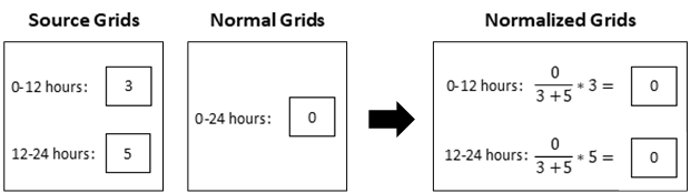
The lower cumulative volume of the normalized grids relative to the PRISM grids is due to how the normalized grid cells are computed. For each normalized grid cell computation, if the cumulative volume during the Normalization Interval of either the source grid or the normal grid is zero, the normalized grid cell value will be zero. This can be seen in the two computation examples below. In Example 1, the cumulative volume of the source grids over the Normalization Interval (1 day) is zero. In Example 2, the cumulative volume of the normal grids over the Normalization Interval (1 day) is zero.

Example 1

Example 2

While small differences in cumulative volume between the corrected, or "normalized," grid and the normal grid may be negligible over the course of a short simulation, these differences in volume can add up through space and time. To see how selecting a longer Normalization Interval reduces the difference in cumulative volume between the normalized grids and the normal grids, add the cumulative precipitation for the "UpTruckeeRv_S10" subbasin for the "WY2017_MRMS_30day_corrected" simulation to the plot by holding the CTRL key, highlighting the "UpTruckeeRv_S10" cumulative precipitation result for all five simulations, and selecting the plot icon on the toolbar. The normalized grids that used a Normalization Interval of 30 days resulted in a similar cumulative precipitation volume over the subbasin as the normal (PRISM) grids at the end of the simulation.

Compare Precipitation Hyetographs

After exploring the differences in cumulative precipitation volumes of the normalized grids, plot the precipitation hyetographs for the "UpTruckeeRv_S10" subbasin for the "WY2017_MRMS_raw" and "WY2017_PRISM_raw" simulations by holding the CTRL key, selecting "Precipitation" in the "UpTruckeeRv_S10" results tree for both simulations, and selecting the plot icon on the toolbar.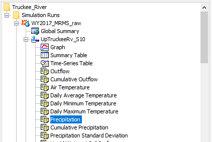

Using the magnifying glass tool on the resulting plot, zoom in to the January 1-6 storm event. Note the slight differences in timing between the MRMS data and the PRISM data. During the 05 Jan: 1200 – 06 Jan: 1200 interval, the PRISM data records a significant amount of precipitation, but the MRMS data records very little. If a Normalization Interval of 1 day was selected, the normalized grid may overestimate the amount of precipitation that fell during the 05 Jan: 1200 – 06 Jan: 1200 interval solely due to the difference in timing between the source and normal grids. However, if the user selected a Normalization Interval that encompassed the entire storm event, such as a 5-day interval, errors due to differences in timing between the source and normal grids could be minimized, since the volume from the entire storm event would be accounted for in the computation.

To view the error created by using a 1-day Normalization Interval, plot precipitation for the "UpTruckeeRv_S10" subbasin for the "WY2017_MRMS_raw," "WY2017_PRISM_raw," and "WY2017_MRMS_1day_corrected," simulations. Using the magnifying glass tool, zoom into the January 1-6 storm event. Note the unreasonably high precipitation value on January 5^th.

The image below shows the hyetograph for the same storm event using a normalized grid with a 5-day Normalization Interval. Because a longer Normalization Interval was used, the shape of the hyetograph of the normalized grid more closely matches the shape of the raw, uncorrected MRMS data.

View Simulated Hydrographs

After gaining a thorough understanding of how the Normalization Interval affects the computation of the normalized grid, view the model results at several different junctions. All three simulations that used a normalized grid more closely replicated the cumulative observed flow at the "Truckee" HEC-HMS model junction when compared to the simulation that used the raw, uncorrected MRMS data.

The image below shows how each simulation replicated observed discharge at the "Truckee" junction during the largest flood event in the simulation. While each normalized simulation offered an improvement over the raw, uncorrected MRMS simulation, the 30-day Normalization Interval resulted in the best fit to the 2017 flood peak.

Discussion Question: What are the risks of selecting a normalization interval that is too large, if any?

Conclusion

Depending on the quality of available gridded precipitation data, creating a normalized precipitation grid may be a necessary step to achieving a well-calibrated, robust HEC-HMS model. When using the Normalizer Tool in HEC-HMS, selecting a reasonable Normalization Interval is a critical step in the normalization process. The Normalization Interval that should be selected for a given HEC-HMS model depends on the size of the watershed, the length of the simulation(s), the purpose of the model, and the gridded data making up the source and normal grids. While the decision largely depends on the modeler's engineering judgment, it is often prudent to select a Normalization Interval that at least spans the duration of a typical rainfall event in the basin. For an event-based model, the Normalization Interval could be set equal to the length of the simulation. For a long-term, continuous model, a weekly or monthly interval could be selected. Longer Normalization Intervals minimize error associated with differences in timing between the source and normal grids and ensure the cumulative volume of the corrected grid closely matches the cumulative volume of the normal grid at the end of the simulation.

This concludes the Workflows for Downloading, Importing and Manipulating Gridded Data workshop.