Download PDF
Download page Example Application with Bald Eagle Creek Watershed.
Example Application with Bald Eagle Creek Watershed
Last Modified: 2024-05-29 10:45:22.099
This page is part of the workshop for Applying the Differential Evolution Optimization Search Method for Single Event Calibration. Return to Introduction to Applying the Differential Evolution Optimization Search Method if you need to download the initial project files.
Create a New Optimization Trial
This section of the tutorial provides a step-by-step procedure for creating a new Optimization Trial within the example project. An iterative approach is presented that attempts to simplify the model due to parameter interactions. Start with the uncalibrated basin model for this example.
- Open the Create an Optimization Trial wizard by selecting the Compute | Create Compute | Optimization Trial menu options.
- Name the new Optimization Trial Example_Trial and click the Next button.

- Select the BaldEagleCk_Sept2004 Basin Model and click the Next button.
- Select the Sept2004 Meteorologic Model and click the Next button.
- The new trial is added to the Optimization Trials folder on the Compute tab of the Watershed Explorer.

- Select the new Optimization Trial to open the Component Editor. Enter a Start Date of 17Sep2004, Start Time of 06:00, End Date of 20Sep2004, and an End Time of 00:00. Select a Time Interval of 15 Minutes.

- Go to the Search tab and choose the Differential Evolution search method. Set the Max Iterations to 100, Tolerance to 0.001, and Population Size to 30. Utilizing an Optimization Trial is an iterative process. You might find that the search converges too quickly or not at all. If this does happen, the Max Iterations should be increased and/or the Tolerance decreased. The Tolerance is an absolute value, and it is applied differently for the selected search methods and objective functions. For the Simplex search method, the search will stop when the change in objective function from one iteration to the next is less than the user defined tolerance. For the Differential Evolution search method, the search will stop when the standard deviation of the objective functions from all parameter sets (usually 30) is less than the tolerance plus the tolerance times the mean objective function. The Population Size determines the number of parameter sets that are traversing the parameter space. A higher population size will result in longer compute times but should aid in the search finding an global optimum parameter set.
- Go to the Objective tab and choose a Goal of Minimization. The Location should be the SpringCk_gage element (this element has observed flow). Select the Discharge Time-Series. The Statistic is the objective function used to evaluate the model's performance (using the simulated and observed flow). Choose the Peak-Weighted RMSE objective function. Make sure the No Transform option is selected for Data Transformation. Then enter a Start Date of 17Sep2004, a Start Time of 06:00, an End Date of 20Sep2004, and an End Time of 00:00. All computed and observed flow values within this time window are used to compute the objective function.

- The next step is to add Parameters to the Optimization Trial. Place the mouse pointer on top of the Optimization Trial's name in the Watershed Explorer. Click the right mouse button and choose the Add Parameter option in the pop-up menu. Add a total of five parameters to the trial.

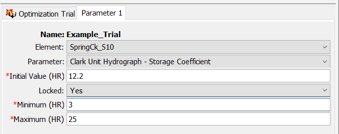
- The figure below shows the Component Editor for Parameter 1. The Element should be set to SpringCk_S10. Once you select this element, the program will build the list of parameters that can be chosen. Select the Clark Unit Hydrograph - Storage Coefficient parameter. The Initial Value is automatically populated using the value from the Basin Model. Make sure Locked is set to No. A value of No means the program will adjust the parameter value during the search. A value of Yes means the program does not vary the parameter during the search. Always modify the Minimum and Maximum values. Do not run an Optimization Trial with the default Minimum and Maximum values. Enter a Minimum value of 3 hours and a Maximum value of 25 hours. These limits are appropriate for the watershed.

- Set Parameter 2 to the Clark Unit Hydrograph - Time of Concentration and enter a Minimum of 3 hours and a Maximum of 25 hours.
- Set Parameter 3 to the Initial and Constant - Constant Rate and enter a Minimum of 0.05 inches/hr and a Maximum of 0.5 inches/hr.
- Set Parameter 4 to the Linear Reservoir - GW 1 Coefficient (1) and enter a Minimum of 3 hours and a Maximum of 25 hours.
- Set Parameter 5 to the Linear Reservoir - GW 1 Reservoirs (1) and enter a Minimum of 1 and a Maximum of 5.
- Run the Optimization Trial. Is will take a couple of minutes to complete. Due to the random nature of the Differential Evolution search method, the number of iterations and optimal parameter values will vary each time the trial is computed. However, if repeatability is required, the seed value can be kept the same between runs to ensure that hte same results are obtained for each run of the same trial. You can try running with a different seed value to see how the results change.
- View results from the optimization trial by selecting the Results tab of the Watershed Explorer, expanding the Optimization Trials folder, and then clicking on the Example_Trial node in the Watershed Explorer.

Below is a plot of observed flow and the computed hydrograph from the optimized model.
The figure below shows the final parameters values from the optimized Basin Model. Your results will be different than those shown below. However, there should be good model agreement with the observed hydrograph.
The figure below shows how the Clark Storage Coefficient progressed across evaluations.
- Currently, there is no option for linking model parameters within an Optimization Trial. For example, linking the GW 1 Coefficient to the Clark Storage Coefficient so that the values are equal to one another is one way to simplify the model. The GW 1 Reservoirs parameter is another parameter within the baseflow method that can be used to change the baseflow response. It is not necessary to adjust both the GW 1 Coefficient and the GW 1 Reservoirs. Locking the GW Coefficient and only adjusting the number of linear reservoirs is a way to simplify the calibration process. Make the following modifications to the Example_Trial optimization trial. You will be locking three of the five parameters to those optimal parameter from the completed trial. The Optimization Trial will be run a second time while only the Constant Loss Rate and GW 1 Reservoirs are adjusted.
- Clark Unit Hydrograph - Storage Coefficient - Set the Initial Value to 12.2 hours and set the Locked option to Yes.
- Clark Unit Hydrograph - Time of Concentration - Set the Initial Value to 15.6 hours and set the Locked option to Yes.
- Linear Reservoir - GW 1 Coefficient (1) - Set the Initial Value to 12.2 hours and set the Locked option to Yes.
- Clark Unit Hydrograph - Storage Coefficient - Set the Initial Value to 12.2 hours and set the Locked option to Yes.
- Run the Example_Trial Optimization Trial a second time. The trial should take a couple of minutes to complete. The following figures show update optimal parameter values and the observed and final computed hydrographs. The optimal Constant Loss Rate is 0.5 inches per hour, which is at the upper end of the reasonable parameter range for this subbasin. Quality of the boundary condition data is always something to consider when modeling historical events and is one reason why it is a good practice to identify reasonable parameter ranges within the optimization trial.


Examine Optimization Trial Results
The figure below shows available results for the DE_NS_Sept2004 Optimization Trial. There are summary tables with information about the trial and optimal parameters, plots showing the objective function value and parameter value for each iteration, and time-series results for basin model elements upstream of the location with observed flow. The time-series results are only for the very last iteration, which includes the final, or optimal, parameter values.

The Optimized Parameters table, shown below, contains the final/optimal parameter values. The initial values are included but do not reflect the starting point for a Differential Evolution search. As mentioned above, the program will randomly identify parameter sets (based on the user defined population size) and then evolve the parameter sets. The Optimized Values in the summary table is the final parameter set that minimized or maximized the objective function.

The figure below shows how the Objective Function varied for each iteration. The plot below shows each evaluation of the objective function for an iteration (for DE with a population size of 30 there are 30 evaluations per iteration). A NNSE of 1 identifies a perfect model - one that is able to exactly reproduce the observed results. In this example, the final parameter set generated an RMSE value of 0.94. The NNSE value is slightly different than the final NSE value of 0.931 (see equation for NNSE here: The Differential Evolution Search Method).

The figure below shows how the Constant Loss Rate parameter varied for the best parameter set across all evaluations. The search method spanned the user defined parameter space before converging on a value of 0.5 inches/hr. This value is at the upper limit of the parameter range, which means boundary condition data should be investigated, other model parameters and parameter interactions should be investigated, and parameter ranges should be investigated.

The figures below show observed (black) and simulated (blue) hydrographs for the SpringCk_gage junction element. The uncalibrated results are shown on the left and the results of the DE_NS_Sept2004 Optimization Trial are shown on the right. The Optimization Trial was able to improve the simulated hydrograph, relative to the observed data, for the single flood event.
 and Final Optimized Parameter Set (right)")
Discussion Question: Compare the results for different optimization runs. Do you think there was any benefit to using the Differential Evolution search method over the Simplex search method in this exercise?
The following table contains initial parameter values, results from the three Differential Evolution Optimization Trials, and results from the Simplex Optimization Trial. There is a variability in the model parameters and the final NS score across the Optimization Trials.
The final NSE can be obtained by opening the Summary Table of the SpringCk_gage junction element.
| Parameter | Initial Parameter Estimate | DE_NS_Sept2004 | DE_PeakRMSE_Sept2004 | DE_SSR_Sept2004 | Simplex_NS_Sept2004 |
|---|---|---|---|---|---|
| Objective Function | Normalized Nash Sutcliffe | Peak-Weighted RMSE | Sum of Squared Residuals | Nash Sutcliffe | |
| Constant Rate (in/hr) | 0.1 | 0.50 | 0.50 | 0.50 | 0.50 |
| Time of Concentration (hr) | 8.09 | 14.15 | 15.90 | 15.85 | 15.00 |
| Storage Coefficient (hr) | 8.09 | 25.00 | 12.38 | 12.32 | 12.26 |
| GW 1 Coefficient (hr) | 8.09 | 17.20 | 7.83 | 11.91 | 23.45 |
| GW 1 Reservoirs | 5 | 2 | 5 | 5 | 5 |
| Final Nash Sutcliffe Score | -5.25 | 0.31 | 0.987 | 0.987 | 0.912 |
Discussion Question: Although you optimized the four hydrologic process parameters, what other aspects of a hydrologic model (that we didn’t touch at all in this workshop) may prevent a “perfect” optimization or calibration?
For this specific model, the Gage Weights meteorology method is an imperfect representation of the way that rainfall is distributed in space and time across the watershed. This problem is called boundary condition uncertainty. Additionally, there is uncertainty about whether the Initial and Constant, Clark UH and Recession Baseflow methods are ideal for representing rainfall-runoff processes in this watershed. This is called model uncertainty. There is also uncertainty about whether the recorded rainfall for the three stations in the meteorological model, as well as the streamflow observations, are the true values. This is called measurement uncertainty. Currently, HEC-HMS is set up to explore parameter uncertainty in hydrologic processes and to a limited degree, boundary conditions. Given that the goal of calibration and optimization is to make your model represent reality, some of these uncertainties remain even after manual or automatic calibration (optimization).
Return to Introduction to Applying the Differential Evolution Optimization Search Method to download the final project files.