Download PDF
Download page The Differential Evolution Search Method.
The Differential Evolution Search Method
Last Modified: 2024-05-29 07:41:18.958
This page is part of the workshop for Applying the Differential Evolution Optimization Search Method for Single Event Calibration. Return to Introduction to Applying the Differential Evolution Optimization Search Method to download the project files.
The HEC-HMS Optimization Trial is meant to be an aid in the calibration process. The modeler should be aware of parameter impacts prior to using this tool. For example, you should understand what happens when the constant loss rate parameter is increased (peak flow should be reduced). The modeler should also have a general idea of reasonable parameter ranges. Subbasin size, slope, land use, and soil information can be used to bound minimum and maximum parameter values.
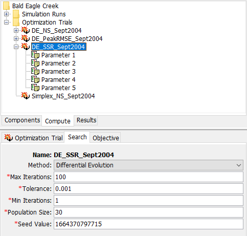
As shown in the figure below, you should see four Optimization Trials when you open the project. The first three trials (their name begins with DE) are configured to use the Differential Evolution search method. Different Objective Functions were selected for the three Optimization Trials configured to use the Differential Evolution search method. The DE_NS_Sept2004 Optimization Trial uses the Normalized Nash Sutcliffe objective function, the DE_PeakRMSE_Sept2004 Optimization Trial uses the Peak-Weighted RMSE objective function, and the DE_SSR_Sept2004 Optimization Trial uses the Sum of Squared Residuals objective function.

Each objective function is unique and was designed to emphasize different aspects when comparing model results to observations. For example, some objective functions emphasize larger flow values while others evaluate model performance with respect to time and volume. The following summary provides additional information about the three objective functions chosen for the tutorial.
- Normalized Nash Sutcliffe - The Nash-Sutcliffe Efficiency (NSE) is a performance measure that compares the variance of the modeled residuals to the variance of the observed flows. It can be thought of as a relative comparison of the noise of the modeled time series to the "signal" contained in the observed time series. The normalized version of the NSE metric rescales it to be on the range [0, 1] where 1 indicates perfect prediction and 0.5 indicates that using the mean of the observed flows is as good of a predictor of the observed time series as the modeled time series. A NNSE value of 0 indicates that there is no information about the observed time series in the modeled one. The normalized statistic is preferred for optimization routines because the lower bound of -\infty for NSE can cause problems with the search. Because higher values of NNSE correspond to better model performance, the NNSE statistic must be maximized when searching for optimal model parameters.
- Peak-Weighted RMSE - The peak-weighted root mean square error is a modification of the root mean square error (RMSE) measure that gives more weight to errors that correspond to larger observed flows. The RMSE measure computes the square-root of the average of the squared model residuals, where the residuals are the difference between the simulated and observed values for a time step. The peak-weighted version multiplies each residual by a weight that increases proportionally to the magnitude of the observed flow for that time step. Smaller values of peak-weighted RMSE indicate better model performance, so it must be used with the minimization goal in an Optimization Trial.
- Sum of Squared Residuals - The sum of squared residuals objective function (sometimes also called the sum of squared errors, similar to linear regression, and has the same interpretation) simply computes the model residual for each time step, squares them, and then adds them all up. It does not have any special weight for any of the residuals. It is related to the regular root mean square error (RMSE) objective function. If you computed the sum of squared residuals, divided by the number of time steps in the model simulation, and then took the square root, you would get the model RMSE. For long-term hydrologic simulation the sum of squared errors can place too much emphasis on periods of low flow or baseflow. Additionally, magnitudes of this objective function are proportional to the length of the simulation time window and can become very large. Smaller values indicate better model performance and this objective function must be used with the minimization goal.
| Objective Function | Formula |
|---|---|
| Normalized Nash-Sutcliffe | NSE=1-\frac{\sum_{i=1}^{n}(q_{i}^{m}-q_{i}^{o})^{2}}{\sum_{i=1}^{n}(q_{i}^{o}-\overline{q^{o}})^{2}}NNSE = \frac{1}{2-NSE} |
| Peak-Weighted RMSE | \sqrt{\frac{1}{n}\sum_{i=1}^{n}(\frac{q_{i}^{o}+\overline{q^{o}}}{2\overline{q^{o}}})(q_{i}^{m}-q_{i}^{o})^{2}} |
| Sum of Squared Residuals | \sum_{i=1}^{n}(q_{i}^{m}-q_{i}^{o})^{2} |
q_{i}^{m} is the modeled flow for timestep i, q_{i}^{o} is the observed flow for timestep i, \overline{q^{o}} is the average observed flow for the objective function time window, and n is the number of model timesteps in the objective function window.
The Differential Evolution search method performs a much more robust search than the Simplex option. The Differential Evolution search method includes an option for the modeler to specify the Population Size (shown below). The Population Size determines the number of parameter sets that traverse the parameter space. In the example shown below, the Population Size is set to 30 and the number of parameters adjusted within a parameter set is set to five. In this example, there are 30 parameter sets, each parameter set includes a unique combination of the five parameter values. The 30 parameter sets move around the parameter space while searching for the optimal parameter set. The variation in the value of the objective function for each of the 30 parameter sets in an iteration is used to assess whether or not the search has converged. The default population size of 30 is generally reasonable for problems with only a few parameters. However, for searches with a very large number of parameters, the recommended population size is 10 * n, where n is the number of parameters.
The Differential Evolution search methods contains logic that determines how the parameter sets move around the parameter space and when the search stops based on the user defined Max Iterations and Tolerance. The Seed Value determines the initial state of the random number generator used in the DE algorithm to generate new population members. The seed is provided so that DE trials are repeatable.

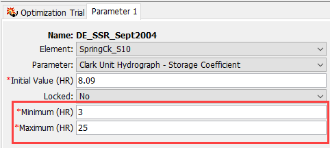
The figure below shows one of the Parameter Component Editors within an Optimization Trial. The Initial Value can be either be left as the default value, obtained from the Basin Model, or the user can enter a different value. All Optimization Trials in the example project have the same initial values specified for similar parameters. The Initial Value has little to no meaning within a Differential Evolution search since parameter sets start with random initial parameter values that span the parameter space.
Initially, the parameter Minimum and Maximum values are set to the default allowable range in HEC-HMS. For example, the Clark Storage Coefficient has a minimum allowable value of 0.02 hours and a maximum allowable value of 1000 hours. Basing the parameter search range on the allowable range within HEC-HMS may result in a model that takes prohibitively long to converge, or may produce unexpected results. It is highly recommended that the minimum and maximum values are edited based on physical characteristics in the watershed. As shown below, the Minimum Clark Storage Coefficient was set to 3 hours and the Maximum Clark Storage Coefficient was set to 25 hours. The same Clark Storage Coefficient Minimum and Maximum values were set for all Optimization Trials in the example project.

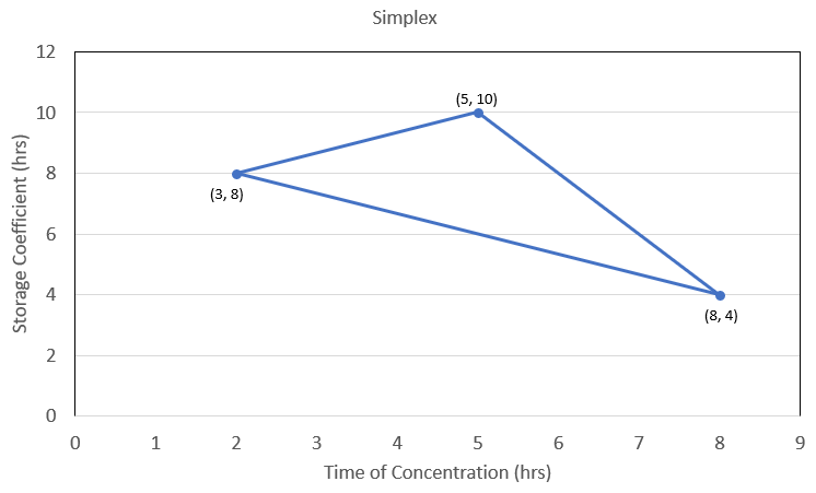
Iterations are treated differently between the Simplex and Differential Evolution search methods. An iteration is one step in the solution process and an evaluation is a computation of the objective function. The evaluation occurs after the model is computed using a unique parameter set. For the Simplex search method, the first iteration has n+1 (n is the number of parameters being adjusted in the trial) evaluations and then iterations after that all have one evaluation. The figure below shows a simple Simplex search with two parameters (Time of Concentration and Storage Coefficient) and the Simplex search has three nodes. A separate simulation is computed for each parameter combination that makes up the Simplex search. The objective function is computed for each of the three simulations. Then the simplex starts moving where only one parameter set is changed, a simulation is computed, and then the new objective function is computed. The new objective function is compared to the objective functions from the existing two nodes and the Simplex determines which node to move towards for the next iteration. More information on the Simplex method can be found here.

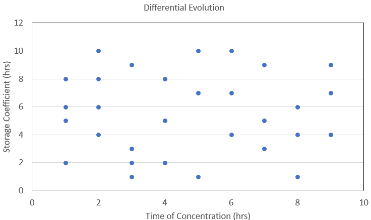
The Population Size is critical for the Differential Evolution search method. It is recommended that a Population Size of 30 is used for most applications. A large enough Population Size is important for ensuring the search covers the full range of plausible parameters, and also for assessing whether or not the search has converged. For the Differential Evolution search method, every iteration has 30 parameter sets (assuming a Population Size of 30), and includes 30 model simulations and then 30 evaluations (computation of the objective function). The Differential Evolution search methods will move the parameter sets around in order to reduce the average objective function using evaluations from all 30 simulations. The figure below shows how the 30 parameter sets might look at the very beginning of a Differential Evolution search (assuming only two parameters being adjusted). The parameter sets will eventually converge through the search and evaluation process. More information on the Differential Evolution method can be found here.

Discussion Question: How do you expect the runtimes to compare between the Differential Evolution and the Simplex search methods? You can test by running the four optimization trials in the example project.
Run times will likely be longer for Optimization Trials that use the Differential Evolution search method. The table below contains the run time for each of the four Optimization Trials in the example project. Run times for trials that use the Differential Evolution search method will vary since part of the parameter search is a random process. Notice the run time for the trial that uses the Simplex search method is much shorter than those trials that use the Differential Evolution search method.
| Optimization Trial | Run Time (seconds) | Number of Evaluations |
|---|---|---|
| DE_NS_Sept2004 | 20 | 26 iterations x 30 population size = 780 |
| DE_PeakRMSE_Sept2004 | 35 | 44 x 30 = 1320 |
| DE_SSR_Sept2004 | 30 | 38 x 30 = 1140 |
| Simplex_NS_Sept2004 | 5 | 109 |
Continue to Example Application with Bald Eagle Creek Watershed.