Last Modified: 2024-05-29 06:15:02.353

This page is part of the tutorial on Applying the Simplex Optimization Search Method for Single Event Calibration. Return to Introduction to Applying the Simplex Optimization Search Method for Single Event Calibration if you need to download the initial project files. 

Set up the observed flow time-series gage and compute Simulation Runs

1. Create a discharge gage in HEC-HMS following information in the Creating Time Series Data tutorial.
   
   

   The observed flow gage will be used by the optimization trial. Results from the simulation will be compared to the observed flow gage and an objective function value will be computed for each iteration during the optimization.

   Name the discharge gage PNXP. The flow data is located in the ...\Simplex_Initial\Optimization_Workshop\data\observe.dss file. Set the pathname to refer to the PNXP flow gage, as shown below.
   
2. Open the Punxsutawney Basin Model by clicking on it in the Watershed Explorer. Select subbasin Mahoning Cr by clicking the element in the Watershed Explorer or in the basin map. 
3. Click on the Options tab in the Component Editor. Select the PNXP discharge gage for the Observed Flow as shown below.
   
4. Create three new Simulation Runs and compute them to make sure they function correctly. All three will have the same Basin Model, Punxsutawney, and the same Meteorologic Model, Specified Gage Wt. Each run will use a different Control Specifications: Apr 94, May 95, and May 96. Use descriptive names for the simulation runs, such as Run Apr 94, Run May 95, and Run May 96, as shown below. Run the simulations and examine the results. You can run the three computes simultaneously through the Compute | Multiple Compute menu. Note that, ideally, you would have a separate Basin Model for each simulation to account for initial conditions (initial baseflow and channel flow).
   
5. Inspect the observed and modeled outflow for Run Apr 94 shown below. Note that the simulated hydrograph do not match the observed flow that well, which is also reflected in the poor calibration statistics in the Summary Table.
   

Set up Optimization Trials

1. Select Compute | Create Compute | Optimization Trial to open the Create an Optimization Trial wizard.
2. The first trial will be used to optimize the model to the April 1994 flood event. Choose a name for the trial (Opt Apr 94), and then select the Punxsutawney basin model, and the Specified Gage Wt meteorologic model. 
3. Select the new Optimization Trial in the Watershed Explorer (go to the Optimization Trials folder on the Compute tab) and move to the Component Editor. Verify that the correct Basin Model and Meteorologic Model are selected. Enter a start and end date that match the control specifications for the Apr 94 simulation and select a Time Interval of 1-hour as shown below.
   
   
4. On the Search tab, select the Simplex method, set a tolerance of 0.01, and a maximum number of iterations of 20 as shown below. The Optimization Trial has a feature where the optimization search will pick up where it left off if maximum number of iterations is increased or if the tolerance is decreased after the simulation reaches the maximum number of iterations or the tolerance is met. 
   
   
5. Switch to the Objective tab. Verify that the objective function the Location is set to the Mahoning Cr subbasin element. Select Minimization as the goal, and set the statistic to Peak-Weighted RMSE.  Make sure the objective function will be evaluated for the entire simulation time window, as shown below.
   
6. Right click on the Opt Apr 94 optimization trial node in the Watershed Explorer and select the Add Parameter menu option, as shown below. A new parameter node will be added to the Watershed Explorer beneath the Opt Apr 94 node. Add three more parameters so there are a total of four parameters. 
   
7. Click on the first parameter node and then move to the Component Editor. Select the Mahoning Cr subbasin in the Element drop-down menu. Select the Clark Unit Hydrograph - Storage Coefficient in the Parameter drop-down menu. 
   
8. Click on the other parameter nodes and select the Clark Unit Hydrograph - Time of Concentration, Initial and Constant - Constant Rate, and Initial and Constant - Initial Loss parameters as shown below.
   
   
   
   Notice the default minimum and maximum parameter ranges. These values are beyond the range of reasonable parameter values for the Mahoning Cr watershed.  
   
   

   In practice, the minimum and maximum values should reflect a reasonable parameter range for the watershed. 

9. Edit the minimum and maximum values before running the Optimization Trial:
   A reasonable range for the Clark Storage Coefficient is between 10 hours and 25 hours,
   Clark Time of Concentration is between 5 hours and 30 hours,
   Constant Loss Rate is between 0.05 inches/hour and 0.4 inches/hour, and
   Initial Loss is between 0 inches and 2 inches.

You can consult Applying HEC-HMS GIS Parameter Estimation Tools for more information on parameter estimation.

Compute Optimization Trial Opt Apr 94 and Examine the Results

1. Use the Compute toolbar to select and compute the Opt Apr 94 Optimization Trial as shown below.
   
   
   Go to the Results tab, expand the Opt Apr 94 node, and select the Objective Function node to open the graph of the objective function values. 
   

   Discussion Question: Based on examining the evolution of the objective function value, do you believe it found the best mix of parameter values?

   Answer...

   The graph below shows the objective function value at each step in the search process for the first optimization trial. Hint: you can click on the Axis tab from the Edit | Plot Properties menu to change the range of X and Y axis.

   

   For a good search evolution, the value of the objective function should decrease.  The search results are not valid if the objective function fails to decrease or fluctuates wildly.  In the above graph, it appears that the objective function is on its way to stabilizing but the value still fluctuates considerably.  In addition, there are several warnings that the compute did not converge within the specified maximum number of iterations, so it is likely that finding the minimum peak-weighted RMSE will require additional iterations. It would be better to make the search tolerance smaller and increase the number of maximum iterations allowed and then recompute the Optimization Trial.

   Note that the number of evaluations is higher than the number of iterations (20), because the Simplex search algorithm performs multiple evaluations of the objective function at each iteration (see User's Manual Model Optimization).

2. You should get a Warning message, WARNING 17101:  Simplex search failed to converge after 20 iterations. This message tells us the optimization could not converge on a final parameter set after 20 iterations (the search tolerance was not met).
3. Increase the maximum number of iterations to 200 and re-run the optimization trial. Notice the compute picks up at iteration 21. 
4. The compute progress window is shown below. Notice the search converged at 106 iterations. 
   
5. Switch to the Results tab of the Watershed Explorer and examine the various results for the optimization trial.
6. Open the Objective Function Summary table to compare the volume, peak flow, and time of peak between the simulated and observed hydrographs. Your results might look slightly different. 
   
7. Open the Optimized Parameters table to examine initial values and optimized values. Notice the final constant loss rate value is 0.05 inches/hour. This value is equal to the minimum value we set as reasonable for the watershed. You could try decreasing the minimum on the Parameter 3 tab and re-running the trial. The model results will improve, but such a low infiltration rate for the watershed indicates some possible deficiencies with the precipitation being applied to the model (i.e. compensating for too little volume in the precipitation data by decreasing the constant loss rate).
   
   
8. You can also assess the model's goodness of fit by simply looking at the time-series graph as shown below. Choose the Observed Data graph. 
   
   

9. The Objective Function graph shows the objective function value at each evaluation in the search process. 

   
   
   The figure below zooms in into the final iterations.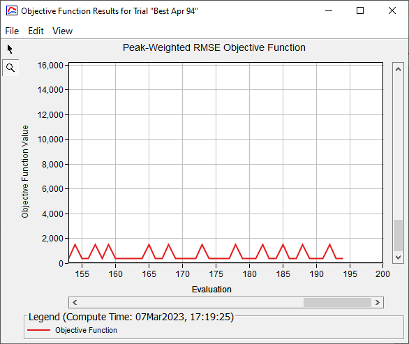 
   
10. You can open a plot of each parameter to see how the parameter value varied for each iteration (parameter from the best node in the simplex). The figure below shows the results for the Clark Unit Hydrograph - Storage Coefficient.
    

Compute Optimization Trials for May 1995 and May 1996 events

1. You can create optimization trials for the other two events by creating a copy of the Opt Apr 94 optimization trial. Be sure you update the start and end date and times used to run the optimization trial and to compute the objective function. Because only one basin model was added to the project, you will need to take care of the initial baseflow for the May 1995 and May 1996 optimization trials (the time window for the 1995 trial should be 17May1995 01:00 to 23May1995 00:00 and the time window for the 1996 trial should be 29Apr1996 01:00 to 07May1996 00:00). Add a fifth parameter to both the Opt May 95 and Opt May 96 optimization trials. Choose the Recession - Initial Discharge parameter and set it to 300 for the Opt May 95 optimization trial and 280 for the Opt May 96 optimization trial as shown below. Also, make sure to Lock the initial baseflow parameter, we do not want the optimization trial to adjust the initial baseflow. 
   

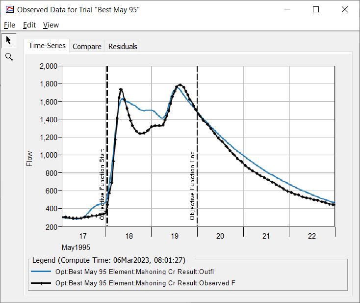
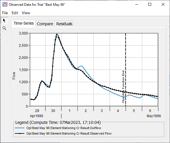
2. Run the two new optimization trials for the May95 and May96 events. Remember to update the time window. You might need to increase the maximum iterations for the trials. Experiment with different objective functions and consider modifying the minimum and maximum parameter values. The figure below shows results from the two additional optimization trials (contained in the final project file below under Best May 95 and Best May 96 results). The final parameter set contains a number of parameters that were at the end of the minimum and maximum range, which indicates additional thought and experimentation are needed.
   
   
   
   
   
   

Proceed to Additional Questions for Applying Simplex Optimization.