Download PDF
Download page Task 3. Determine Ordinal Association Between Variables in R.
Task 3. Determine Ordinal Association Between Variables in R
Return to Task 2. Extract Extremal Events in HEC-SSP.

What is Rank Correlation?
Rank correlation measures the statistical dependence between two variables based on their ranks, rather than their actual values. Using ranks leads to scale invariant estimates. Kendall's \tau, or more formally the Kendall rank correlation coefficient, was developed by Maurice Kendall in 1938. \tau is computed using the number of concordant and discordant pairs.
A concordant pair describes a pair of observations where both variables (X and Y) move in the same direction:
- Both increase: (X₁ < X₂ AND Y₁ < Y₂)
- Both decrease: (X₁ > X₂ AND Y₁ > Y₂)
A discordant pair describes a pair of observations where variables move in opposite directions:
- X increases, Y decreases: (X₁ < X₂ AND Y₁ > Y₂)
- X decreases, Y increases: (X₁ > X₂ AND Y₁ < Y₂)
\tau is computed using the following formula:
| \tau = \frac {C - D} {\binom {n}{2}} |
where C is the number of concordant pairs, D is the number of discordant pairs, and n is the number of paired observations. {\binom {n}{2}} is the binomial coefficient and is equivalent to \frac {n(n-1)}{2}. Kendall's \tau ranges from -1 to 1, inclusive. A value of 1 indicates perfect positive correlation (rankings agree perfectly), -1 indicates perfect negative correlation (rankings are the exact reverse), and 0 indicates no correlation/independence between the rankings.
Computation of Kendall's tau for Philippi, WV Flow and Precipitation Data
The computation of \tau has not yet been implemented in HEC-Neptune.
We plan to migrate the Correlation Analysis from HEC-SSP to HEC-Neptune and implement Kendall's \tau in HEC-Neptune next year!
The R MultiHazard package Kendall_Lag function computes \tau and associated p-values over a range of lags. This function can be used to identify near coincident events that maximize rank association with extremal events. A sample script showing how to apply the function is available here.
We will quantify the ordinal association between extreme events in one variable and near-coincident events in the other using Kendall’s \tau. The analysis will be performed in both directions to address the following questions:
What time lag between an extreme precipitation event and a high-flow event produces the strongest association?
What time lag between an extreme river-flow event and a large precipitation event produces the strongest association?
For each direction, we will evaluate a range of time lags (-5 to +5 days). The lag associated with the highest Kendall’s tau will be interpreted as the most likely temporal offset between the extreme event and its near-coincident counterpart.
The \tau and p-values are plotted and tabulated below. In the plot, black circles indicate that the p-value is less than the significance level of 0.05 at that lag and white circles (not shown here) indicate that the p-value is greater than the significance level of 0.05 at that lag. A small p-value tells you that dependence is statistically detectable at that lag; however, it does not tell you the strength of the dependence.
Note that the range of lags that should be considered is dependent on the variables/system being studied.
Dependence for Extremal Precipitation Events and Near Coincident Flow Events

| Lag (days) | -5 | -4 | -3 | -2 | -1 | 0 | +1 | +2 | +3 | +4 | +5 |
|---|---|---|---|---|---|---|---|---|---|---|---|
\tau | 0.023 | 0.065 | -0.010 | -0.045 | -0.123 | 0.107 | 0.218 | -0.077 | 0.027 | -0.029 | 0.105 |
The strongest computed dependence was a rank correlation of 0.218 at a +1-day lag, indicating that near coincident flows occurring one day after extremal precipitation events had the highest association.
Dependence for Extremal Flow Events and Near Coincident Precipitation Events

| Lag (days) | -5 | -4 | -3 | -2 | -1 | 0 | +1 | +2 | +3 | +4 | +5 |
|---|---|---|---|---|---|---|---|---|---|---|---|
\tau | 0.026 | 0.108 | -0.068 | 0.073 | -0.029 | 0.343 | -0.116 | -0.071 | -0.076 | -0.129 | 0.039 |
The strongest computed dependence was a rank correlation of 0.343 at a 0-day lag, indicating that near coincident flows occurring one day after extremal precipitation events had the highest association.
We now have 2 sets of event pairs (shown in the image below):
- Annual peak flow events and the near coincident precipitation events, and
- Annual peak precipitation events and near coincident flow events.
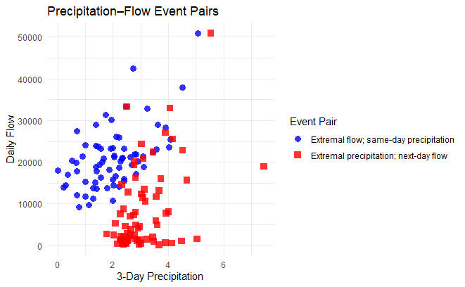
The event pairs are provided in 2 files titled "flow_dominant.csv" and "precipitation_doiminant.csv" on this page.
Question 2. Based on the Kendall's \tau values computed in Task 3, do you think it's reasonable to consider precipitation and flow events independent?
The \tau values of 0.218 and 0.343 indicate weak to moderate positive dependence between precipitation and flow. While the correlation is not particularly strong, it is high enough that assuming the two variables are independent as done in the Coincident Frequency Analysis tutorial (Task 1 - Coincident Frequency Analysis in HEC-SSP) may be questionable.
A copula-based approach does not require the user to assume a particular level of dependence. The copula is fitted directly to the observed data and can represent the dependence structure between precipitation and flow, regardless of whether the relationship is weak, moderate, or strong.
In addition, the dependence between extremal flows and near coincident precipitation is higher than between extremal precipitation and near coincident flows.
Continue to Task 4. Fit Marginal Distributions in HEC-SSP.