Download PDF
Download page New Features.
New Features
HEC-RAS Beta 5 Features
Pipes (Beta)
Side Inlets, Top Inlets, and Manholes
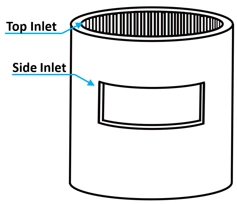
Side Inlets are a new type of surface connection to the Pipe Network in which the inlet opening is oriented vertically on the node. The primary use case of Side Inlets is for modeling of detention pond overflow structures with inlets on the side. In addition, Side Inlets can be used to more accurately model curb opening inlets which were previous modeled as Drop Inlets in HEC-RAS. Side Inlets are defined by selecting an opening shape (Box, Circular), dimensions, weir and orifice coefficients, an invert elevation, and attaching it to a node. Weir or orifice equations are used to compute flow into or out of the inlet based on hydraulic conditions.
Drop Inlets have been replaced by Top Inlets, a new Layer under Nodes in the RAS Mapper Tree. This change allows a Top Inlet to be defined in the Top Inlet attribute table once, and then attached to many nodes throughout the Pipe Network. Existing Drop Inlets will be converted to Top Inlets automatically, but the old Drop Inlet columns remain in the node attribute table only for reference and can be deleted.
Top and Side Inlets have a new Surcharge Only option which prevents surface flow from entering the Pipe Network at the inlet, but allows flow to surcharge out of the network and on to the surface. This new option can be used to model manholes with covers. 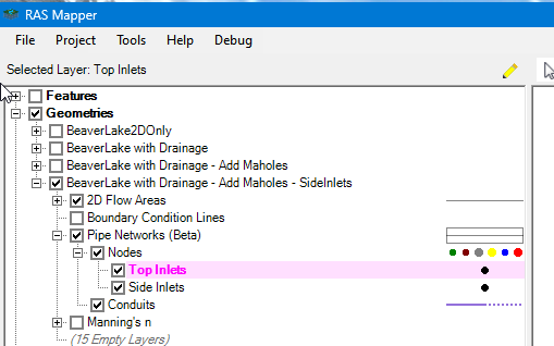
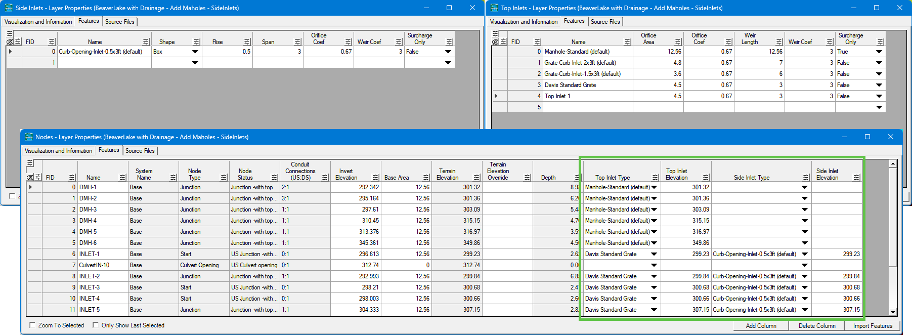
The animation below demonstrates how to see where each inlet type is located in the Pipe Network by selecting the inlet from attribute table.
Pipe Network Gates
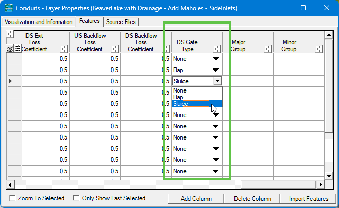
HEC-RAS now has the capability to model sluice style gate inside of Pipe Networks. Adding a sluice gate can be accomplished in the Conduits attribute table using the DS Gate Type field as shown below. Gates can be used on the ends of Pipe Networks controlling flows from the surface, or they can be used inside of Pipe Networks to control flows from node to node.
Once a sluice gate is added to the geometry, the controls for the gate are set in Unsteady Flow Data Editor. The user can define controls using Rules, Time Series, or Elevation Control in the same way they are defined for other 1D and 2D structures in HEC-RAS. Gates locations (Flap and Sluice) are shown in RAS Mapper near the end of the conduit, and they also appear in the conduit profile plot. 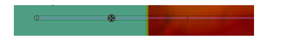
Pipe Network Culvert Opening Inflow Improvements
Culvert Opening Nodes are now computing more accurate inflows into the Pipe Network under various hydraulic conditions. Inflows into Culvert Opening nodes are now using inlet control conditions to allow flow into the network. Improvements to weir flow computations for buried pipes were also implemented. More details can be found in the Hydraulic Reference Manual at a later date.
Linux
HEC-RAS now has the capability to run the Linux compiled computation engines using Windows Subsystem for Linux (WSL). The WSL system and linux (e.g. Ubuntu) must be installed to use this new capability. Running Linux engines from within windows is intended testing and to assist preparing Monte-Carlo type runs on cloud services. The overhead initiating each WSL process makes simulations runtimes longer than native windows computation engines. This new option to use the Linux computation engines via WSL will only be visible if those files are installed with the special Linux installation package.

Numerical Reproducibility
HEC-RAS has added options to increase model reproducibility with parallelized computations. The User Interface offers three options with varying levels of numerical reproducibility. The default is the fastest which provides reproducibility with reasonable tolerances for hydraulic modeling. The other two options provide stricter levels of reproducibility with increasing runtime costs. For more information see Numerical Reproducibility.

Run Multiple Plans
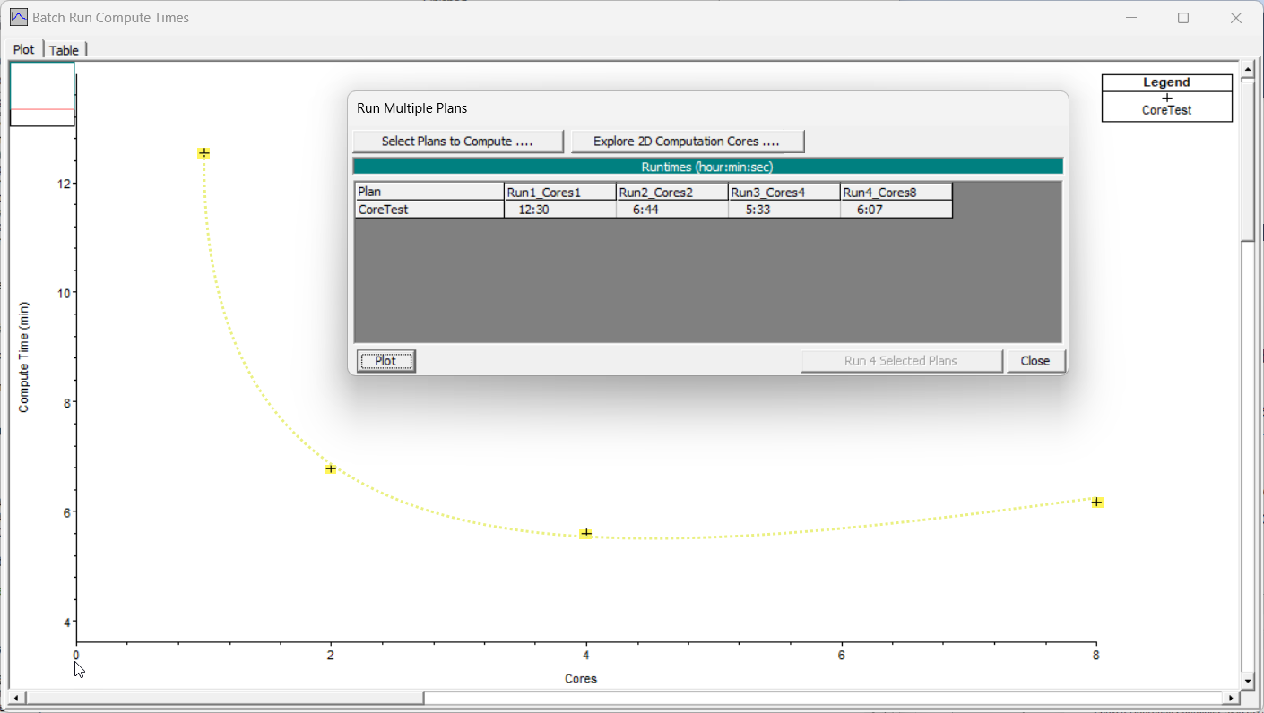
Investigation into the number of solver cores that would be most efficient for a model simulation for has been added in HEC-RAS under the Run Multiple Plans option. This option allows you to quickly set up multiple simulations with a different number of processors to see the effect on run times consolidated into a single table. For more information see Run Multiple Plans.
Option for Energy Grade for Weir Equation at Internal SA/2D Connections
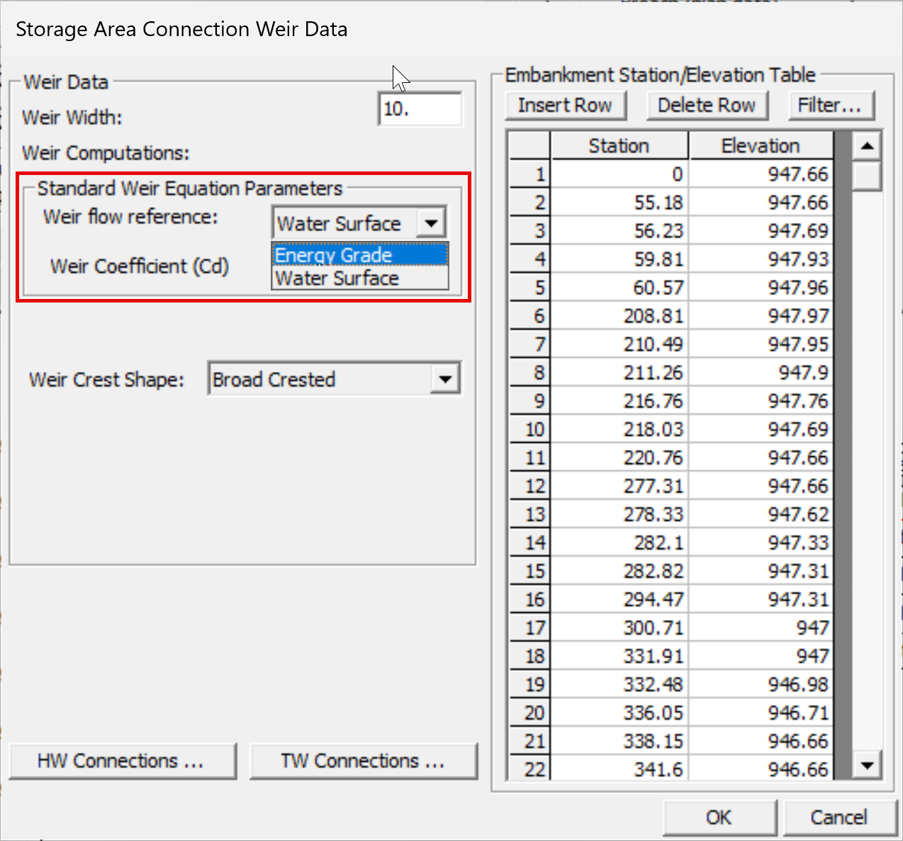
The headwater elevation for the weir flow equation for 2D structures (i.e. SA/2D Connections) now has the option to use the Energy Grade (rather than the water surface). The example below shows the Storage Area Connection Weir Data editor and the option to select Energy Grade or Water Surface for the weir equation at a lateral structure. In previous versions of HEC-RAS allowed for the user to select either Energy Grade or Water Surface for the weir equation at lateral structures connected to storage areas and 2D flow areas. HEC-RAS 6.7 Beta 5 adds this same option to internal SA/2D Connections.
2D Bridge Scour Export Tools
This Beta version of 6.7 includes a beta version of the new 2D Bridge Scour tools. The tool has added:
- Output variables required to use the Federal Highway Administration's Hydraulic toolbox
- An automated tool to export 2D hydraulics from HEC-RAS reference lines directly into a hydraulic toolbox file
- Detailed (and evolving) documentation on how to use 2D HEC-RAS results with the Bridge Scour Toolbox
Plotting
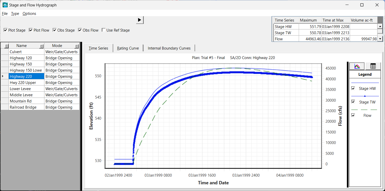
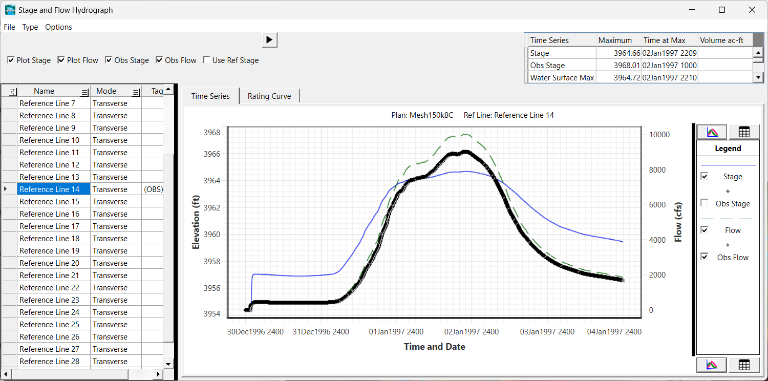
The Stage and Flow Hydrograph plotter has undergone major changes. The Stage and Flow Hydrograph Plot now has option buttons to see all plots for all computational node types in one window. This includes for time series data plots, profile plots, hydraulic table property plots, and breach information. This output will continue to improve with 6.7 Beta 5. To learn more about what is available, check out the User's Manual.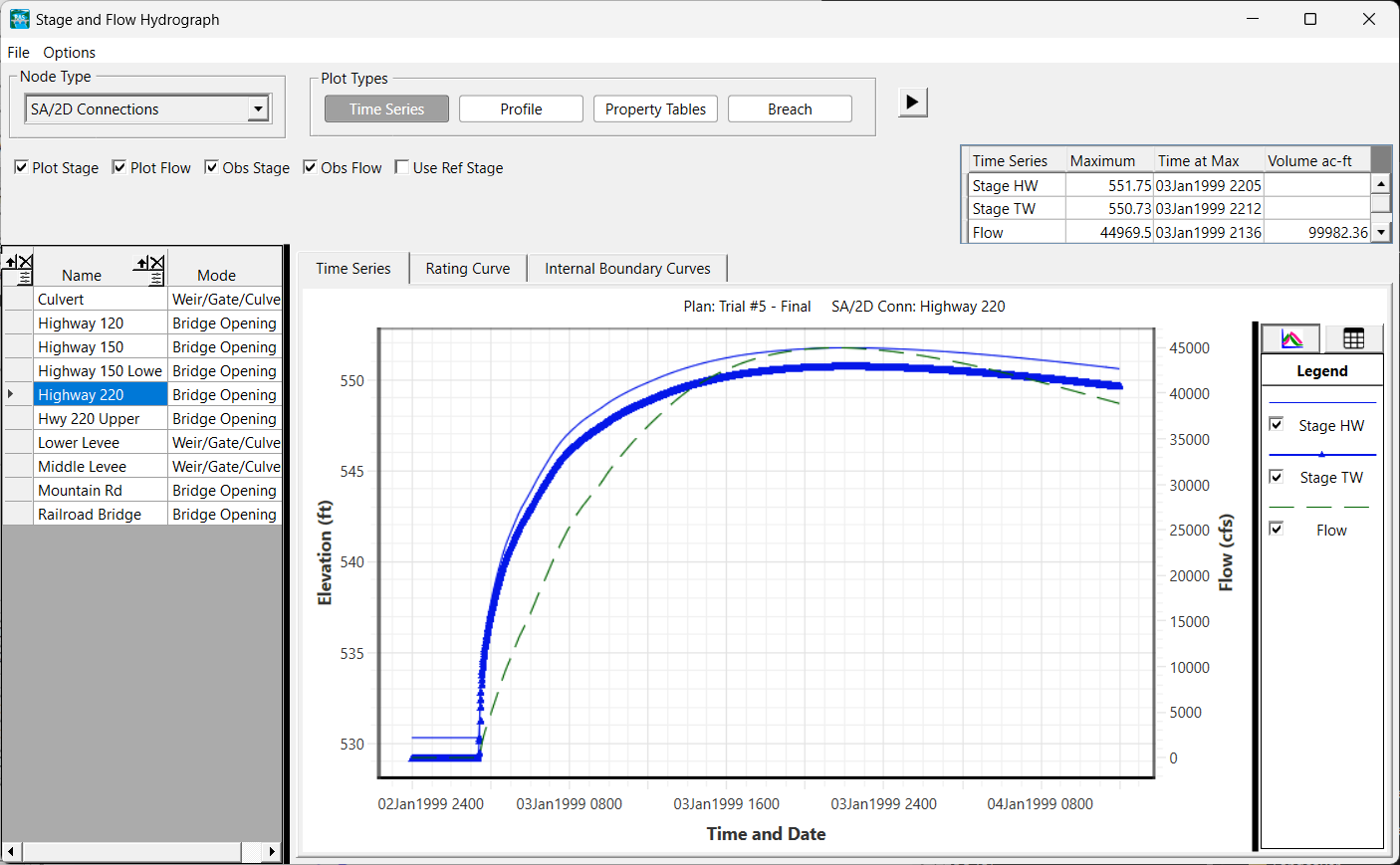
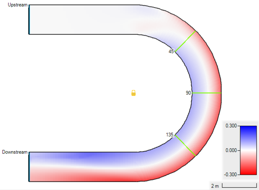
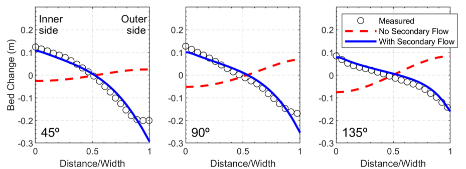
Secondary Flow Effects in 2D Sediment
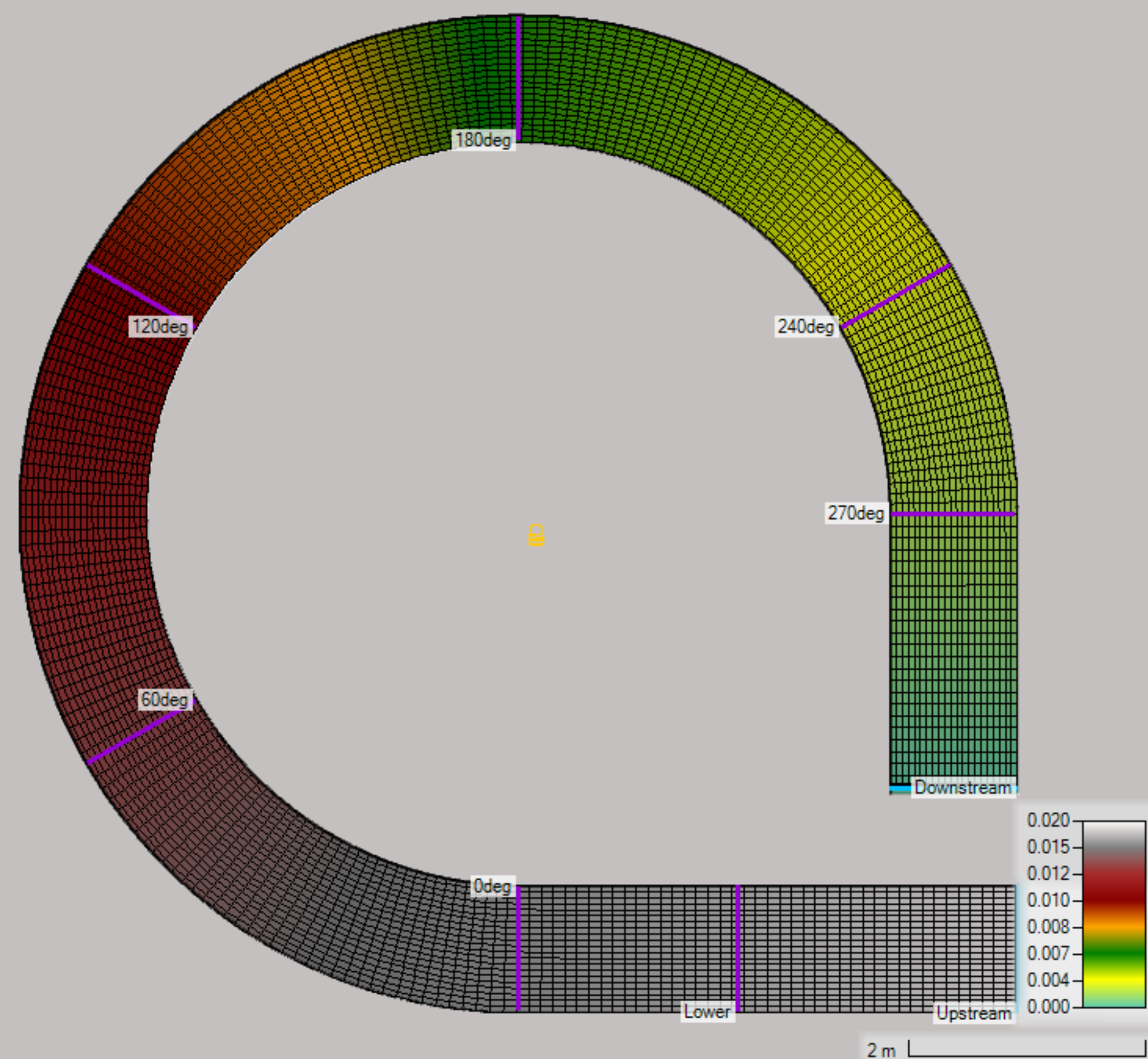
HEC-RAS 6.7 Beta 5 includes the effects of secondary flow in 2D sediment transport (see 2D Sediment Transport). Secondary flow at river bends is caused by the balance between the outward centrifugal acceleration and the inward pressure gradient and produces a flow towards the outer bank near the surface and towards the inner bank near the bed. The effects of secondary flow on sediment transport are to produce a suspended sediment dispersive flux towards the inner side of the bend as well as a deviation of the bed-load transport towards the inner side of the bend. These effects are balanced by the bed-slope effects. A an example validation result the figures below show computational results for the laboratory flume study of Koch and Folkstra (1980). The flume channel has a rectangular cross-section with a width of 1.7 m and a longitudinal bedslope is 0.18%. The ratio of the mean radius of curvature to the width is 2.5 m which represents a sharply curved channel. A constant upstream flow of 0.17 m3/s and downstream stage of 0.2 m were applied. The sediment median grain size is 0.78 m. The lower left figure shows a map of the final bed change including the effects of secondary flow. The computed bed change shows erosion on the outer side of the bend and deposition on the inner side. The lower right figure shows a comparison of the bed change with and without secondary flow compared to laboratory measurements. The bathymetry was compared at three transects at angles of 45, 90, and 135 degrees along the bend. The HEC-RAS results compare well with measurements.
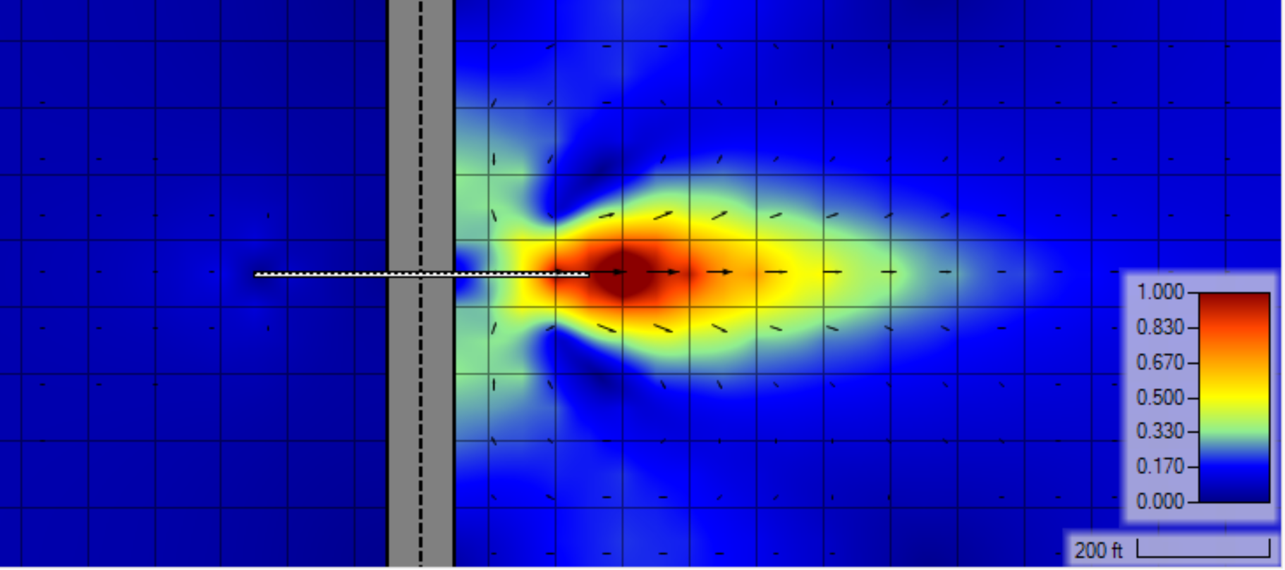
Momentum from Georeferenced Culverts
Momentum from georeferenced culvert outflows is now included in 2D Flow Areas with Shallow Water Equations. Georeferenced culverts are culverts for which the coordinates of the culvert layout are specified. The outflow from culverts introduces momentum into the 2D Flow Area cells. The feature does not work for non-Georeferenced culverts or when using the Diffusion Wave Equation. The figure below shows an example of a lateral structure with geo-referenced culvert with flow from left to right. The culvert outflow produces a local circulation including a water jet and water entrainment near the lateral structure.
The direction of the flow is taken into account. The momentum calculations treat the culvert momentum semi-implicitly and has been shown to have good stability for most applications. Culverts can be submerged or above water in which case a correction is applied to reduce the momentum for plunging flow. For more details on the hydraulic calculations see Hydraulic Reference Manual - Culvert Flow into 2D Flow Areas.
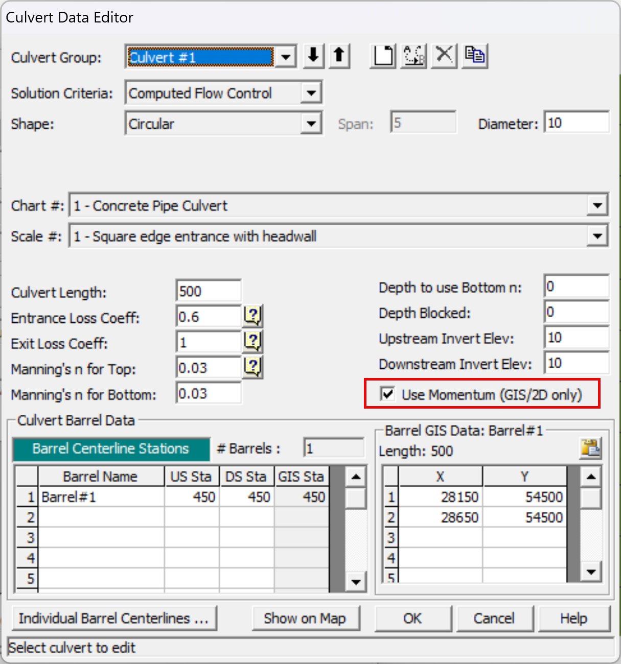
The feature is not on by default and has to be turned on per lateral structure in the Culvert Data editor by clicking on the checkbox Use Momentum (GIS/2D only) (see figure below).
HEC-RAS Beta 4 Features
CPU Affinity
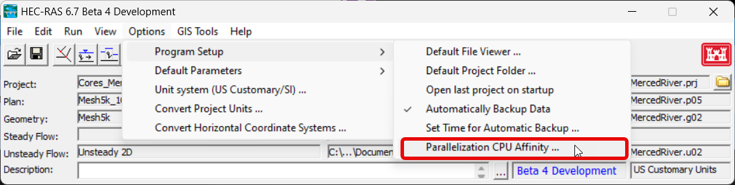
The addition of "efficiency cores" added to new CPUs now allows computers to more efficiently perform computations at the expense of speed performance. The previous method in HEC-RAS for determining the available number of processing cores did not differentiate between "performance cores" ("p-cores") and "efficiency cores" ("e-cores") which could result in slower run times. With HEC-RAS 6.7 Beta 4, RAS implements a new method for determining the availability of p-cores and limiting the solver to just those cores during 2D simulations. To enable CPU options, select the Options | Program Setup | Parallelization CPU Affinity menu item.
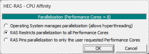
CPU Affinity options allow the user to choose to have the operating system to manage parallelization or have RAS to just use the "p-cores" during the unsteady flow computations. The default option is to restrict computations to just the "p-cores". A more detailed discussion about CPU Affinity options in HEC-RAS is provided in the HEC-RAS Users Manual.
When using the "All Available" option for number of cores, previous versions of HEC-RAS did not differentiate between performance and efficiency cores. With Version 6.7, HEC-RAS will limit computations to just the Performance Cores if "All Available" is selected. Best performance can be achieved by manually setting the number of cores per 2D Flow Area.
Secondary Flow (Beta)
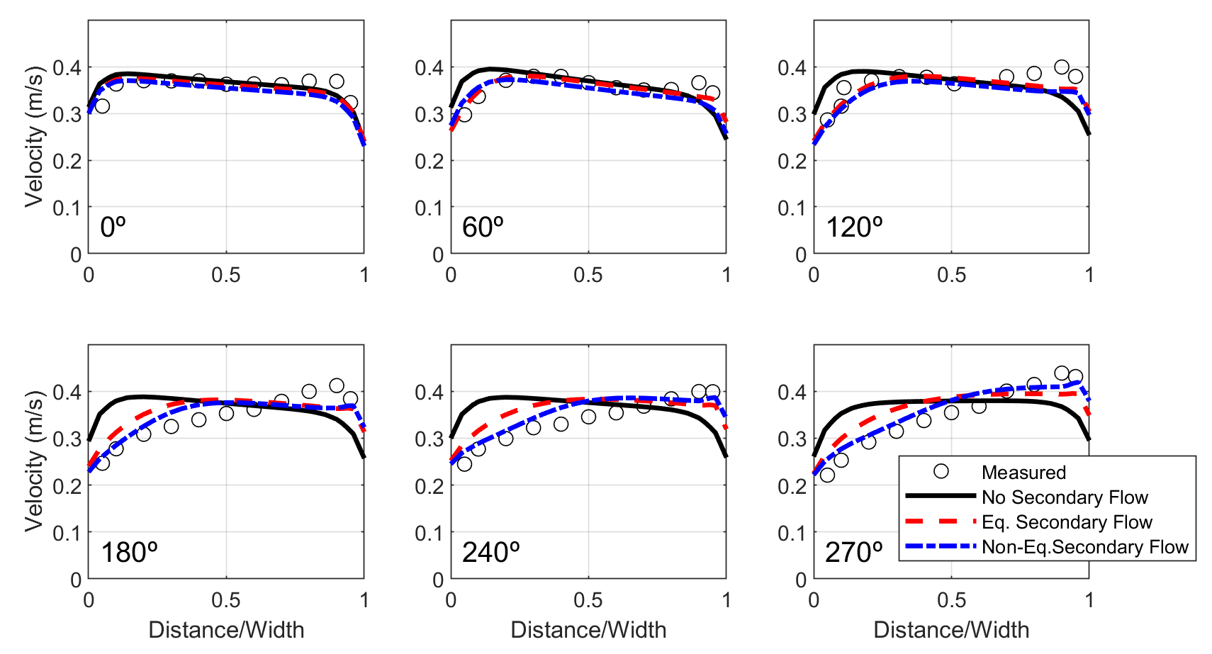
In river bends, the balance between the outward centrifugal acceleration and the inward pressure gradient produces a secondary flow which flows towards the outer bank near the surface and towards the inner bank near the bed. A new feature has been added to simulate the effect of helical or secondary flow around river bends in the shallow water equations. The approach used in HEC-RAS closely follows that from Delft3D-FLOW and has both equilibrium and non-equilibrium formulations. Example results are shown here for the flume experiments from Steffler (1984). The computational grid was generated in HEC-RAS 2025 and has 21 cells across the channel. A comparison of HEC-RAS velocity profiles at different transects along the flume is shown below. The results are computed without secondary flow, with equilibrium secondary flow and with non-equilibrium secondary flow. Overall, the HEC-RAS results with secondary flow show good agreement with measurements. This non-equilibrium secondary flow approach is more accurate, especially at the downstream end of the flume, but the equilibrium approach offers a good compromise between accuracy and computational efficiency since it is approximately 40% faster in this case.
Secondary flow corrections for 2D sediment transport are currently under development and will be released in the next version of HEC-RAS.
Structure Plots
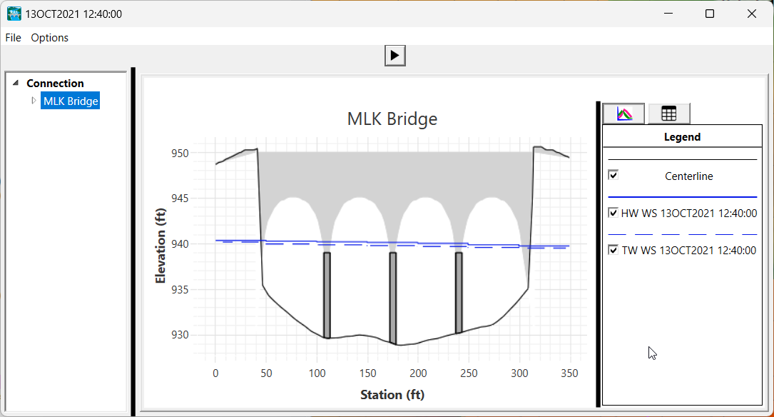
Profile plots now add hydraulic structures within the profile to show the low chord relative to the water surface profile.
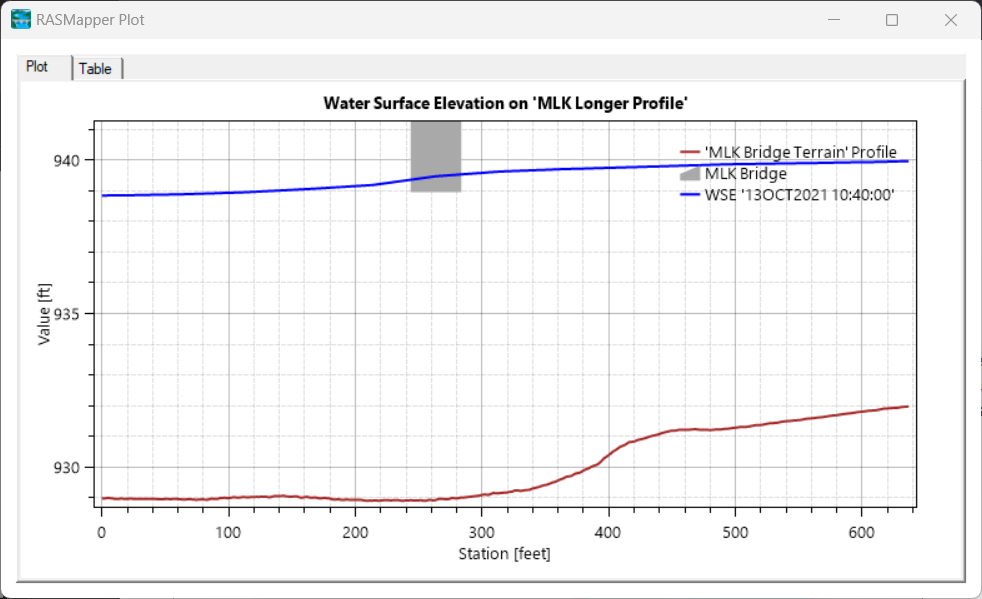
Structure plotting for hydraulic structures show the effective structure with headwater and tailwater water surface elevations.
Time Series Plot
The hydrograph plot now incorporate a table for more efficient access to plots of the same type. As shown in the figure below, all of the 2D Connections are directly available in the list to the left of the plot. This workflow is available for Boundary Conditions, Reference Lines, 2D Faces, etc. Below is an example of the hydrograph plot for multiple bridges and culvert openings.
Another example for Reference Lines with Observed data, is shown below.
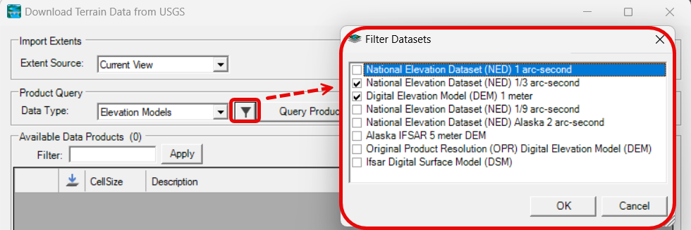
USGS Data Download
The USGS NED data server has been inconsistently working to automatically download data. Experimentation has shown that attempting to query of multiple data sources was inconsistently failing (more than 2 sources fails). HEC-RAS now has the ability to filter by individual data dataset to explicit query the data of interest. This will allow the download of specific resolution data (1m, Original, etc.) and flexibility to work around server side request issues. A blank query (returning all data sources) is default.
New Tutorials
HEC-RAS Beta 2 and Beta 3 Features
Bridges
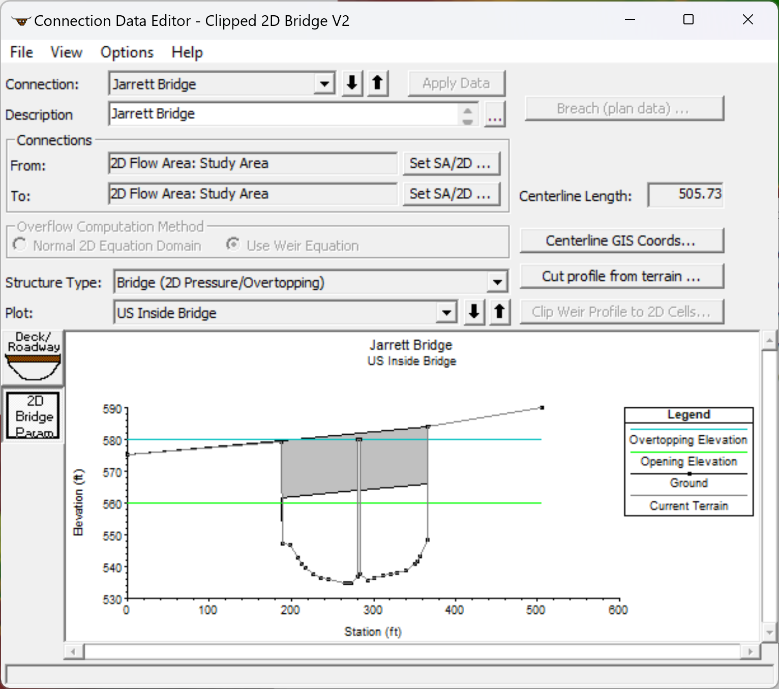
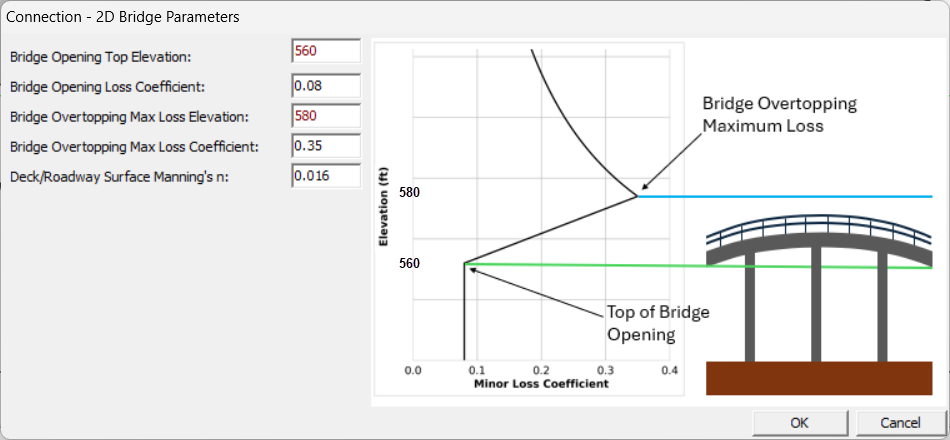
2D Bridges - Pressurized and Overtopping Flow
A new methodology of solving flow through a bridge in 2D models has been added. This feature is designed for detailed hydraulic simulations of flow through bridges. The method solves separate 2D horizontal flow equations through the bridge opening and above the bridge deck. The method can be applied to low flow, pressurized flow, and overtopping. The method includes a simple approach for adding minor losses not captured by the 2D hydraulics by means of a simple energy loss coefficient. Use of this method requires that the bridge piers and abutments are included in the terrain model, along with a detailed mesh with faces capturing the terrain details.
1D Bridges - Momentum Method Improvement
The momentum method for low flow through bridges (1D bridges and 2D models with bridges of type "1DFamily of Rating Curves") has been improved to handle bridges where the upstream and downstream cross section areas differ significantly. In such cases, the Legacy method could result in poor hydraulic tables for the low flow portion of the curves, as shown in figure below.
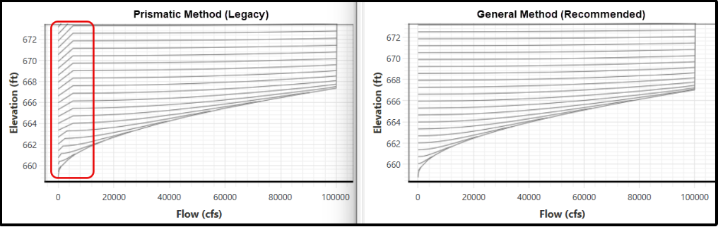
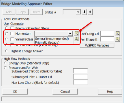
The old method is referred to now as "Prismatic (Legacy)" and the new method as "General (Recommended)". You can read more on Low Flow Momentum Bridge Computations in the Hydraulic Reference Manual and is easily accessed by clicking the Help button on the Bridge Modeling Approach editor, as shown below.
RAS Mapper
Addition of Reference Line output and access to Results has been improved for 6.7 Beta 2.
Menu Reorganization and Access to Results
Simulation results can be accessed by right-clicking on the Plan and selecting the Plot Results Profile or Show Results Table menu items.
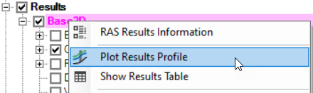
- Plot Results Profile will invoke a plot window with Reference Lines as the selected output locations.
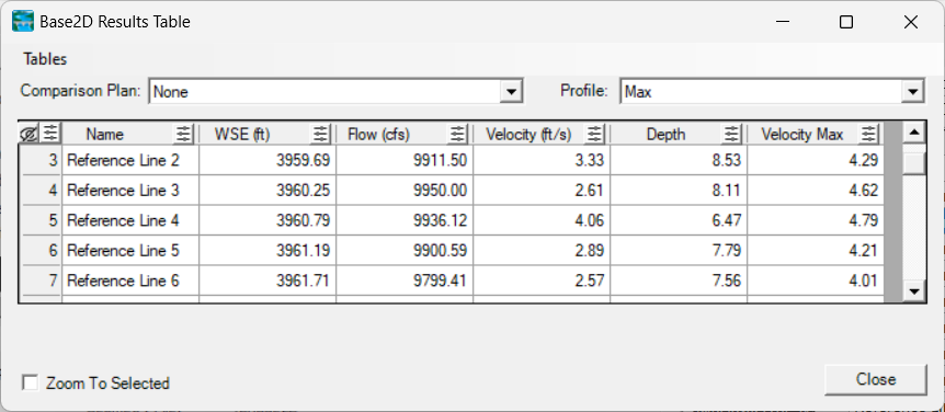
- Show Results Table will invoke a table of computed hydraulic variables for each Reference Line.
The access to Results from the Map Window have also been improved. There are now two main context menu headings accessible from a right-click: Results and Mapping Results. These options are available when the Plan is selected in the Layers List (on the left of the Map Window).
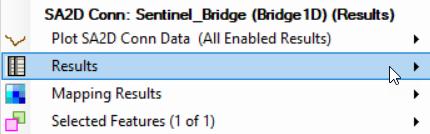
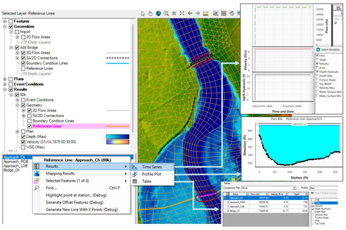
- Results provides access to information from the computation engine written to the results file (.p##.hdf). This includes such plots such as Time Series Plots at cells and faces and Time Series Plots and Profile Plots at Reference Locations.

.")
.")
- Mapping Results provide interpolated values from the the Map using the selected Water Surface Rendering Mode. As the name implies, these results are coming from mapped results that are interpolated from the the computed cell values.
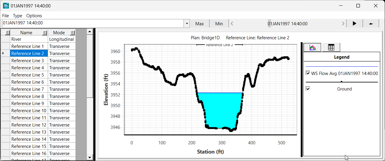
New Average Variables Plotting Capabilities for Reference Lines
HEC added new average and max variables to the reference lines including average and max, velocity, and hydraulic depth as well as the flow, area, top width and friction slope of the flow across the reference line (variables used for bridge scour calculations). The 6.7 Beta 2 also includes tools to access these results directly from mapper, in summary tables, and as classic cross section plots.
Sediment, Mud, and Debris Features and Documentation
Rating Curve Calculator Connected to new USGS Data (and new plots)
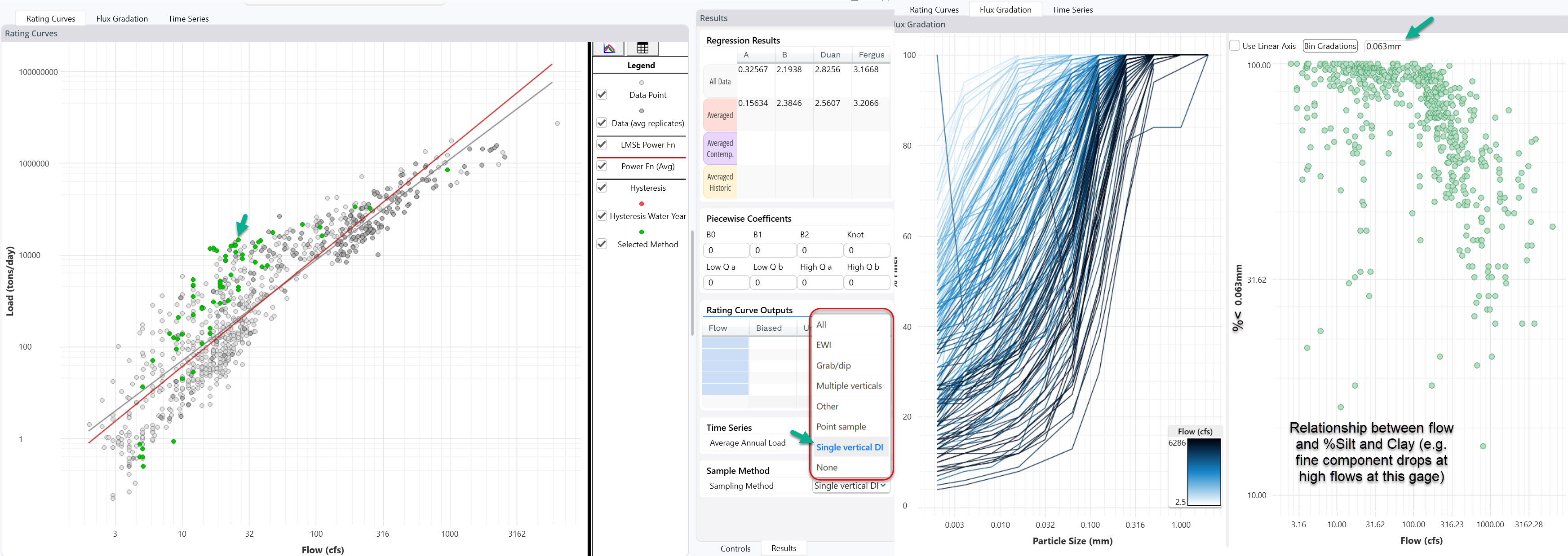
HEC updated the sediment rating curve calculator to read the new water quality format (the USGS discontinued the old format making the tool inoperable). The USGS still has not made the text search functionality available, but users can apply the tool if they have a gage number for now. HEC also added two new analyses: view data by sampling type and a % fine mode in the grain size analysis (because many gages have more sand-silt split data than grain size distributions).
New Tutorials, Guides, and Classes
- New 1D Steady Flow Lecture Videos
- BSTEM (Bank Failure) Tutorial
- Variable Concentration Mud and Debris Modeling Guide
- 2D Connection Overflow Equation Selection (Weir vs 2D) and Mesh Best Practices Guide
 Modeling Weir in RAS (video)
HEC-RAS 6.7 Beta Features
Pipe Network Features
Pipe Networks - New Conduit Shapes
Pipe networks now allows for many conduit shapes beyond circular. The full list of conduit shapes now includes: circular; box (rectangular); arch; low profile arch; high profile arch; ellipse (horizontal and vertical); semi-circular, and ConSpan (see figure below).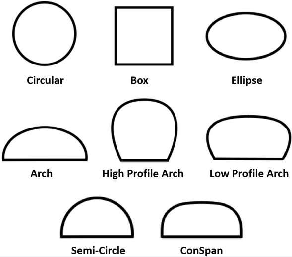
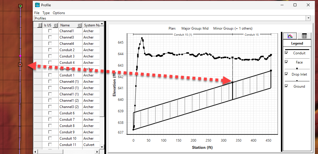
Pipe Networks - Results Profile Plot Improvements
Several improvements have been made in the pipe network results profile plot to make for easier visualization and analysis including, the addition of flow, velocity, and critical depth profile plots along the conduit, and easier access to the animation control bar.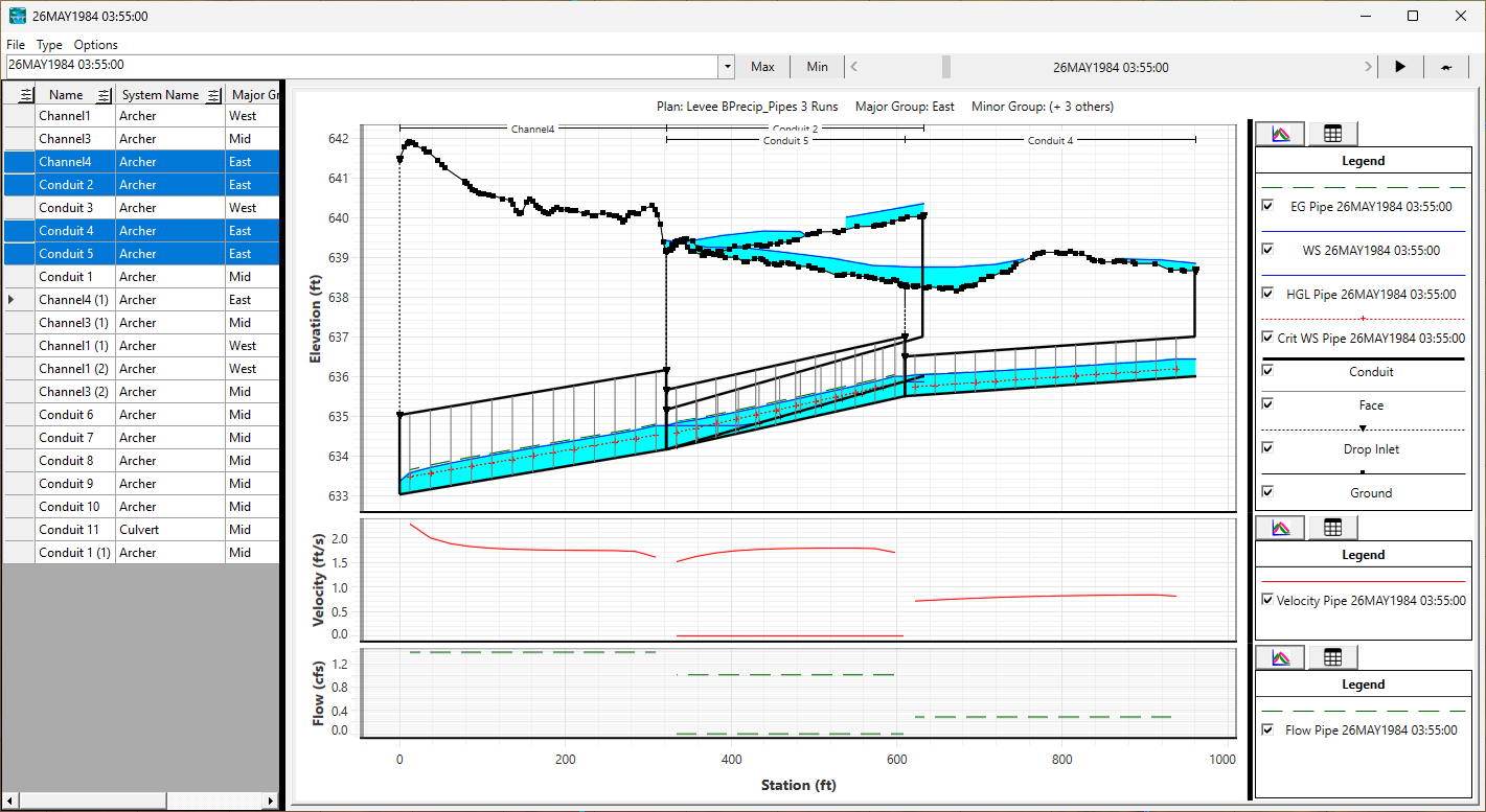
Saved Lists are now available in the pipe network profile plot allowing users to save and quickly plot groups of conduits.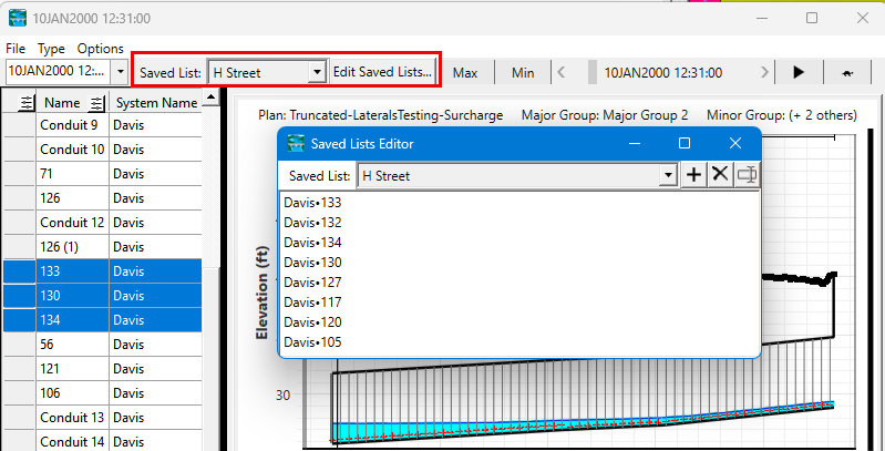
Pipe Networks - Property Tables and Cross-Section View
User's can now visualize the conduit cross-sections and property tables from the Hydraulic Tables menu as shown below.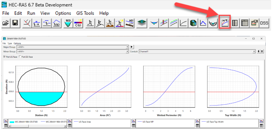
Pipe Networks - Speed Draw Mode
In order to help draw pipe networks more quickly, the Speed Draw mode automatically places nodes at the ends of newly finished conduits. To turn on Speed Draw mode check the box in the conduit editing tool bar, then nodes will be placed at the ends of each newly completed conduits if one does not exist there already.
Pipe Networks - Split Selected Conduit and Add Node
With the Split Selected tool users can choose where to split a conduit, and at that location a new node will placed along with two new conduits that maintain the properties of the existing conduit.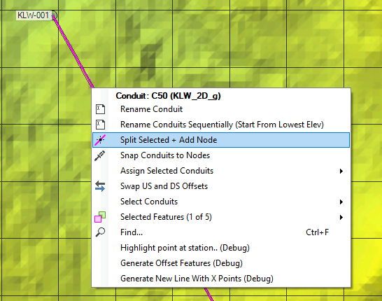
Sediment, Mud, and Debris Features and Documentation
Automatic Hydraulic Updates for Morphological Acceleration
The Morphological Acceleration Factor provides the opportunity to explore 2D sediment transport and morphological change at a fraction of the full run times. But previous versions required users to compress their flow time-series manually (inverse to the morphological acceleration) to conserve time. This was an awkward and confusing process that also distorted results temporally.
Version 6.7 can now automate that process, applying the morphological acceleration factor to the specified time series, and applying the compression automatically for both input and output.

BSTEM (Bank Failure) Update and Tutorial
HEC fixed several bugs in the USDA-ARS bank stability and toe erosion model (BSTEM) included in the 1D, mobile-bed model - particularly in the multiple-layer algorithms.
As part of this testing and development process, we also developed a BSTEM tutorial.
Variable Concentration Mud and Debris Modeling: Features and Guide
The fixed-bed, non-Newtonian, approach to mud and debris flow modeling is a good level of complexity for many geophysical flows. But it is limited to a single concentration (spatially and temporally).
Some applications require mixing (e.g. dam failure into clear water or tributary debris flow into a clear-water mainstem) or downgradient deposition.
HEC has added several methods in recent versions intended to make variable-concentration, non-Newtonian modeling easier.
We developed a guide that describes several approaches to variable concentration non-Newtonian modeling at different levels of complexity, leveraging several of these new tools (Concentration Only Routing, Hindered Settling, Erodibility Multiplier, Global Depositional Threshold) and creative repurposing of existing tools (Excess Shear cohesive equation and Mixture Fall Velocity methods added for flocculation).