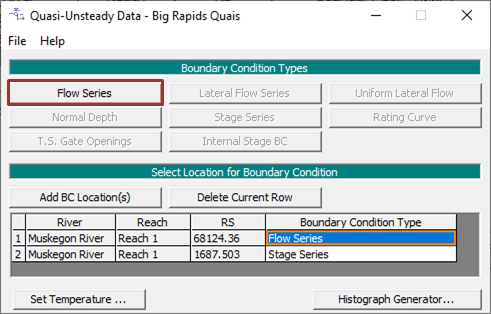
HEC-RAS requires external (upstream and downstream) boundary conditions to run sediment analyses. The Quasi-Unsteady Flow editor automatically includes entries for external boundary cross sections, requiring boundary conditions.

The quasi-unsteady flow model has multiple boundary condition options for downstream and internal boundary conditions, but only one Upstream Boundary Option: the Flow Series.

Select and define a Flow Series for each upstream boundary.

Click the blank Boundary Condition Type field associated with the upstream node and then press the Flow Series button to open the Flow Series editor.

Flow Series

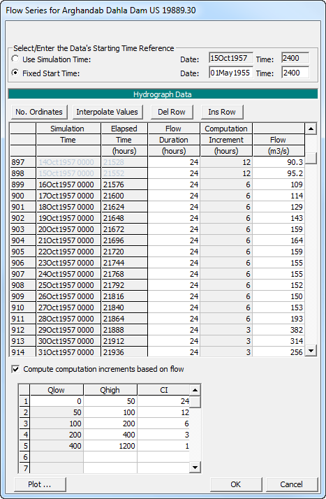
Define upstream boundary flow in the Flow Series editor, depicted in the figure below. The Quasi-Unsteady Flow series editor shares the look and feel of the Unsteady Flow series editor with a few important differences. The time reference conventions are the same as unsteady flow (DDMMMYYYY). Most sediment models tie the flow series to a Fixed Start Time reference. This feature ties historical records or synthetic future records to a fixed start date, allowing simulation windows that include all or any part of the record. For example, in the figure below the historical record starts at 01May1955 2400 but the simulation starts on 15Oct1957 2400. The shaded dates indicate that those flows are outside the simulation window (defined in the plan editor described here).

One of the unique (and sometimes confusing) details of the quasi-unsteady editor is that each time step and flow has two time steps associated with it: a Flow Duration and a Computational Increment.  The Flow Duration has the resolution of the flow data (e.g. daily flows have 24 hour durations) while the Computation Increment is the actual computational time step, at which HEC-RAS recomputes the hydraulic backwater and simulates transport. 

Flow Duration:

The flow duration is a constant flow input increment. It does not control the model time step. For example, if flow data are from a daily USGS flow gage, flow durations would be 24 hours, regardless of the computational time step applied to the sediment model. The Computational Increment (e.g. hydraulic and sediment transport time step) can be smaller than the Flow Duration, but not larger.  Therefore, the Flow Duration is also the maximum time step. 

Modeling Note: Develop Longer Flow Durations for Low Flow Periods With the Histograph Generator

Modelers often want to use very large (multi-day) time steps during low flow, low transport seasons.  In these cases, users can combine multiple flow durations into one, and run the long duration with an average flow and a single computational increment.  (e.g. run a week of baseflow with insignificant transport as a single flow duration of 168 hours with a 168 hour computation increment).  However, averaging flow does not average sediment.  Running a sediment model with average flow introduces sediment errors, usually overpredicting the sediment load.  If loads are during the averaged flow periods are significant, the Histograph Generator, will compute load-scaled time series with sediment-averaged flows that conserve sediment mass.

Specify Flow Durations in the first column of the flow editor (in hours). Values can be copied from Excel and pasted into the Flow Series Editor with the Ctrl+C and Ctrl+V commands, but all of the destinations cells must be selected. (Note: all destination cells can be selected by clicking on the heading. Users can also populate the table (particularly if all the durations are the same) by dragging a value (hover over the bottom right corner of the cell to get cross hairs to drag values) or populating the first and last value and pressing the Interpolate Values button.

Quasi-unsteady flow can handle irregular (varying) time steps, allowing coarse time steps

Flow durations for different boundary conditions do not need to match. If boundary conditions have different time steps (flow durations or computational increments) HEC-RAS will compute and use the smallest time step common to all.
The Flow Series editor defaults to 100 rows. Almost all sediment studies require more flow records. Press the No. Ordinates (number of ordinates) button to customize the Flow Series length up to about 40,000 flows.

If the model requires more than 40,000 flows, either combine low flows into longer durations (possibly using the Histograph Generator tool) or consider running the model in two phases, hotstarting the geometry and bed gradation (see Hotstart section below) .

Computational Increment:

The Computational Increment subdivides the Flow Duration. The quasi-unsteady model computes new steady flow profiles at each computational increment, applying the hydraulic parameters over this time step. This approach assumes bed geometry does not change enough between computational increments to alter hydrodynamics appreciably.

Sediment transport is highly non-liner. Most transport and bed change is concentrated in relatively brief periods of high flow, and flood events are often highly dynamic. Large quasi-unsteady time steps (e.g. 24 hours or more) are often sufficient for low flow periods with little bed change. However, moderate to high flows can change channel geometry quickly, undermining the assumption that the hydrodynamics are the same throughout a large time step. Therefore, moderate to high flows require smaller computational increments.

Model stability is very sensitive to computational increment. If the simulation window reports "Model fills with sediment" when the model fails, the computational increment associated with that flow duration is probably too large. If channel geometry is updated too infrequently (i.e. if the computational increment is too large), too much material could be eroded or deposited in a time step, causing the model to over correct in the next time step, generating oscillations and model instabilities.

For example, the first two flow records in the figure 'Flow Series Editor' shown above, (02 and 03 January) are daily flow records with 24 hour computational increments. Therefore, HEC-RAS will only compute hydraulic parameters once over these days. However, the third- and fourth-time steps (ending 04Jan and 05Jan) have daily flow durations but are subdivided into multiple steps. HEC-RAS will update the hydraulics four times during the third flow record (every 6 hours, based on the 6 hour computational increment) and will update hydraulics 24 times (every hour, for the fourth and fifth flows), at the beginning of each 1-hour computation increment.

Modeling Note: Computational Increments Drive Run Times and Model Stability

While smaller computation increments will increase run time, re-computing geometry and hydraulics too infrequently (e.g. computation increments that are too large) is the most common source of model instability.

Automate Computational Increments (Optional)

It is often useful to apply a consistent flow-computational increment (CI) relationship to the entire flow series, particularly when trying to optimize the increment for a long flow series. HEC-RAS will automatically populate computational increments with user specified flow ranges. Click the Compute Computation Increment Based on Flow check box (below). This will open an editor to associate consecutive, non-overlapping flow ranges with computational increments. The feature also grays out the computational increment column, because it populates automatically. The computational increments persist and become editable if the user turns the Compute computation increments based on flow off (i.e. uncheck the check box), but the tool will overwrite any existing computational increments if it is turned on.

Modeling Note

If your flow time series includes flows lower than the smallest flow of higher than the largest flow in your automated computational increment, HEC-RAS will automatically use the Computational increment associated with the lowest or highest range respectively. (Note: this is new in version 6.0. Previous versions returned an error)

Fixed or Simulation Start Time?

Most HEC-RAS time series editors aske users to Select/Enter the Data's Starting Time Reference. This is one of the places in HEC-RAS where the default is usually not the best practice. Use Simulation Time is the default. In this method, the time series is always relative in time. The first record will always adopt the starting time in the Simulation time window. So in the figure below, the simulation starts on 10Jan1984, so the default time reference (bottom right of the figure) automatically assigns that time stamp to the first flow (the Simulation Time in quasi-unsteady marks the end of the time step, so it shows 11Jan).

However, apart from experimental studies with set start times or synthetic hydrographs, flow data are almost always temporally fixed. The example on the left in the figure above shows a Fixed Start Time that begins on 01Jan. Now the simulation that starts on 10Jan starts on the 10^th daily record. The Fixed Start Time has two main advantages:

1. First, using fixed start times allows users to simply enter their complete data time series for different boundary conditions without trimming them all to the same start time.
   
   
2. Second, Fixed Start Times give modelers a lot of flexibility in the simulations. By fixing time series, modelers can shift the simulation time window to simulate a wet-r-dry decade, a three-day flood, a full period of record that is longer than the project window, multiple calibration periods, or other sensitivity/calibration/credibility tests without editing the flow file.

Therefore, the Fixed Start Time is the appropriate data format for most sediment models, whether the data are historical or synthetic future.

Warning: Select the radio button when setting a fixed start time

A common error in HEC-RAS modeling involves setting a fixed start time but forgetting to select it with the radio button. This can be a problem in models with many boundary conditions. After adding all the flow boundary conditions, go in to each one and make sure the Fixed Start Time is not only specified, but also selected.

Using DSS Flow Data for a Quasi-Unsteady Simulation

Previous versions (before 6.0) of HEC-RAS could not use DSS files to define quasi-unsteady flow boundaries. Current versions can define quasi-unsteady flows with a regular time-step DSS flow record. Defining flows with a DSS record helps coordinate the sediment transport model with other HEC software, flow data bases, and allows HEC's stochastic engine (HEC-WAT) to sample hydrologic realizations and automate stochastic simulations that evaluate the role of hydrologic uncertainty on quasi-unsteady sediment transport.

However, irregular time steps are important in long term sediment transport models. Daily flow time steps are often too coarse for floods, requiring modelers to subdivide daily flows into smaller computational increments for high flows. Therefore, the Compute Computation Increments Based on Flow feature works with regular time-step DSS flows, assigning irregular computational increments to each flow, based on its magnitude. This gives users control over an irregular computational time step even if they import a regular time step DSS record.

Users can also use the histography generator to convert a regular time-step DSS file into an irregular time step quasi-unsteady flow file based on equal sediment mass flux.