Download PDF
Download page Mixed Flow Quasi-Unsteady Sediment Simulation.
Mixed Flow Quasi-Unsteady Sediment Simulation
Overview of Mixed Flow Sediment Options
Open channel flow has two stable states: sub-critical (deeper & slower) and super-critical (shallower and faster). Most natural channel flows are sub-critical. However, some steep transitions can pass through critical flow (e.g. a headcut, in-channel mining pit, or the edge of a reservoir delta during a dam removal or flush). Earlier derisions of quasi-unsteady hydraulics would default to critical depth for anything that might be super-critical.
Steady flow has three flow regimes, sub-critical, super-critical, and mixed. Unsteady will compute mixed flow by default (though the 1D unsteady flow engine usually develops instabilities as water surface elevations approach critical depth). The 2D finite volume engine is more stable through a mixed flow transition, so a simplified 2D model is an option for mixed-flow sediment. But in recent versions HEC has also added mixed flow to the more stable quasi-unsteady engine.
Boundary Condition Assumption
The quasi-unsteady engine simulates a series of steady flows. Therefore each quasi-unsteady time step requires the boundary conditions of a steady-state profile. The steady-flow mixed flow regime calculations require a minimum of three external boundary conditions, a downstream stage, an upstream flow and an upstream stage. Because each simulation makes an upstream and downstream pass at the calculations and then selects a flow regime at each cross section based on the maximum specific force. But a full time series of upstream stage (in addition to flow and downstream stage) is an unrealistic data requirement. Therefore, the quasi-unsteady algorithm follows the steady flow, mixed regime approach precisely, but on the downstream, super-critical, computational pass during each time step, it begins with a calculated critical depth at the upstream cross section. This allows users to select mixed quasi-unsteady flow without requiring any additional boundary conditions. Checking the Mixed Flow box on the Quasi-Unsteady simulation window is all that HEC-RAS requires to start a mixed flow run. However, the Mixed Flow simulation will add run time, as the steady flow computation has to make two computational passes per time step.

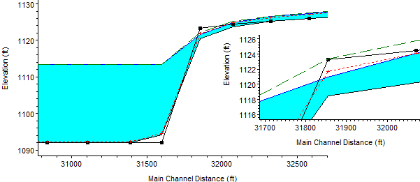
Example Result
This model applied the mixed flow approach to a head cut that formed after channel mining. The mixed flow hydraulics computed super-critical flow (Froude # > 1) at the crest of the mining pit and increased the total erosion along the headcut.


Sediment Transport Functions Were Not Developed for Super Critical Regimes
Sediment transport functions should be used over the range of sediment properties and hydrodynamic settings they were developed under. And even in those conditions, they can generate widely divergent answers. But none of the sediment transport functions in HEC-RAS were developed for super-critical flow regimes. This feature presses all of the transport functions out of their intended range. We do not have much experience with the functions in this range, but our hypothesis is that it would favor the more theoretical equations over the more empirical equations. But, regardless of the equation selected, sediment results in super-critical regimes should be considered even more uncertain than other sediment results, which makes calibration even more important for studies that use this feature.
Critical Depth Options
The Quasi-unsteady simulation editor retains the two critical depth features from the steady flow simulation editor, because both will affect the results, run time, and/or visualization.

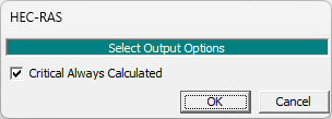
The Critical Depth Output Option requests a critical depth calculation at every cross section whether HEC-RAS computes it or not. HEC-RAS will save computation time by not computing critical depth if it doesn't need to, by default, but it can be helpful to see critical depth at all of the cross sections.
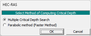
Second, HEC-RAS has two methods to compute critical depth that represent a tradeoff between run time and accuracy. The default Parabolic Method approximates critical depth by fitting a polynomial to the specific energy curve. This method works reasonably well for most situations, and is substantially faster. The Multiple Critical Depth Search (also called the Secant Method) performs better in situations where the specific energy curves has local minimums, usually when hydraulic thresholds (e.g. bridges, ineffective flow areas, "levees") introduce discontinuities in conveyance or wetted parameter. The Secant Method subdivides the specific energy curves into regions to make sure it finds the global maximum. This method avoids local-minimum errors, but requires more run time.
Steady flow simulations rarely take long enough that the increased run time of the more detailed critical depth calculation, or calculating critical depth at every cross section increases run time enough to matter. But long-term sediment models can call the steady flow engine tens- or hundreds-of-thousands of times, making these accuracy-run time tradeoffs important.