Download PDF
Download page Output Level.
Output Level
The sediment model in HEC-RAS can generate over a hundred result variables. Many of those variables also have sub-results as they are sub-divided by grain class or reported in either mass and volume. Output files can get very large, and the variable list can be unwieldy, when the calibration phase of a model study often evaluates the same three-to-five plots each run.
Therefore, HEC-RAS includes several tools to control the number of variables reported. The user can control the number of output variables, as well as the frequency at which HEC-RAS will generate them in the Sediment Output Options. The Output Level controls the variables output. Select and Output Level from one (four variables) to six (all variables) at the top of the Sediment Output Options window (below). The default output level is 4, which reports 14 variables at each time step. It is often advantageous to increase the level to six, to see all variables. However, sediment output files can get very large, because they output most variables by grain class, increasing file size by about an order of magnitude. Multi-Gigabyte sediment output files are common, but more output does not increase run time appreciably. Select the output level that optimizes the tradeoff between file size management and information required. The variables associated with each level are included in the following section, including and detailed description of many of the variables.

Modeling Note: Be Careful with Instantaneous Results
Any variable that does not have a Cum label is instantaneous. This is unproblematic for instantaneous variables like shear stress or concentration. However, if users do not choose to output every computation increment, mass flux and change variables will not balance and may miss peaks.
Table: Variables associated with each level of output.
Level 1
Level | Variables | |
Level 1 | Invert Elevation (ft) (m) – The elevation of the channel invert of each cross section – the lowest elevation between the channel banks. Invert Change (ft) (m) – The total change in the invert (the lowest elevation station-elevation point between the bank stations) since the beginning of the simulation. Water Surface (ft) (m) – The water surface elevation at that at the cross section during the time step. Mass (or Volume) Bed Change Cum*: All (tons or ft3) (tonnes or m3) – Cumulative mass or volume added (+) or removed (-) from the control volume since the beginning of the simulation. Only Total in Level 1. For Grain Class specific results, increase to level 4. Long. Cum Mass (or Volume) Change (tons or ft3) (tonnes or m3)– The cumulative mass or volume change (see above) since the beginning of the simulation, summed from the upstream cross section in that reach. (e.g. the sum of the mass change for all of the cross sections between the selected XS and the upstream reach limit). The total value at the downstream XS of the reach is equal to the total mass change of the entire reach. This is a powerful model evaluation tool metric modelers become familiar with it. Only Total in Level 1. For Grain Class specific results, increase to level 4. |
*Cum = Cumulative – results are summed since the beginning of the run
Modeling Note: Incremental Results Only Reflect Computation Increment
The Mass or Volume parameters track sediment mass movement through each control volume. Users can view discrete mass variables for each specified computation increment, as snapshots in time, or as cumulative masses, accumulated over time (CUM). All mass variables can also be viewed as volumes. Incremental mass or volume results, that is output at intervals coarser than the computation increment (by default results are reported every 10 computation increments) can cause confusion. Because these mass results only reflect the single computation increment output, they will not sum to the cumulative result.Level 2
Level 2 | All Variables from Level 1. Level 2 includes additional hydraulic parameters used in the sediment model (which may be different than the HEC-RAS hydraulic output). Flow (cfs) (m3/s) – The flow at the cross section at the time step. Velocity (ft/s) (m/s) – Average channel** velocity – the flow between the channel banks divided by the area of eht channel. Shear Stress (lb/ft2) (Pa or N/m2)– Channel average shear stress. The is the computational shear stress from the sediment computations: |
**Because the sediment model uses channel hydraulics in the transport equations, the hydraulic output usually reflect channel hydraulics (i.e. only the hydraulics between the channel banks, excluding overbank flows). The channel shear and velocity are usually substantially higher than the cross section averages
♱The computed sediment shear stress can differ from the shear stress displayed in the general, HEC-RAS hydraulic output. The HEC-RAS hydraulics do not compute shear stress, so the shear stress visualizations outside the sediment editors are computed on the fly from other hydraulic parameters. The hydraulic shear visualization is computed from
| \tau = \gamma_w \times R \times S_f = \gamma_w \times \frac{Area}{P_w} \times \left( \frac{Flow}{K} \right) |
Where Pw is the wetted perimeter and K is conveyance. Note, the hydraulic display also computes the channel, overbanks, and full cross section, while the computational sediment shear is for the channel only.
Level 3
Level 3 | Level 3 includes gradation data, some additional hydraulic parameters, and a sediment flux term. Note: All particle sizes are always in mm in input and output even if the model is in US customary units.d10 Cover/Subsurface/ Inactive Layers (mm) d90 Cover/Subsurface/ Inactive Layers (mm) Effective Depth (ft) – A weighted average depth that often reflects the total cross section shape and change more than the invert change. This is also used in the shear stress equation. where: Di is the average water depth in each cross section element (the trapezoid subsection "i" associated with each station elevation point), Ai is the area of that element, and n is the number of subsections. Effective Width (f–) - Effective width is the comparable channel width that preserves cross section area given the Effective Depth - (Units: ft or m) Manning's n Channel (s/ft1/3 or s/m1/3) - This is the Manning's n value in the channel (between the channel banks). If the channel has laterally varied n values, it is the composite channel n. It can be dynamic in time if the water surface weights the composite n-values differently, if there is a flow, or seasonal n value dependency, or if a dynamic, sediment bed roughness predictor is selected. Unlike the Chezy equation the manning coefficient is not dimensionless. Froude Number Channel - The Froude number in the channel (between the channel banks). HEC-RAS computes the Froude Number as: where: Qch is the flow in the channel, Wchis the top width of the channel, g is the acceleration of gravity and Ach is the area of the channel, where the channel is the portion of the cross section between the channel banks. Mass (Vol) Dredge Cum (tons or ft3) (tonnes or m3) – The total mass or volume dredged from that cross section since the beginning of the simulation. Note: This variable will only populate if the model has a dredging event. This output has also changed from version 5, which only reported instantaneous results. See and example in the Dredging section. |

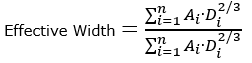
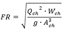
Table: Bed Layer Mass/Volume and Gradation Index Variables by bed mixing algorithm.
Thomas (Ex5) and | Active Layer |
Cover (Mass/Vol) (GC) | Active (Mass/Vol) (GC) |
Subsurface (Mass/Vol) (GC) | Inactive (Mass/Vol) (GC) |
Inactive (Mass/Vol) (GC) | |
Cover Thickness | Active Thickness |
Subsurface Thickness | Inactive Thickness |
Inactive Thickness | |
d10,d16, d50, d84, d90 Cover | d10,d16, d50, d84, d90 Active |
d10,d16, d50, d84, d90 Subsurface | d10,d16, d50, d84, d90 Inactive |
d10,d16, d50, d84, d90 Inactive |
Level 4
Level 4 | Includes variables from levels 1-3. This is the default level, so it includes the most used variables. Starting in level 4, the Mass and Volume results include total and each active grain class.+ This includes new Mass and Volume variables in this level as well as mass and volume variables (e.g. Mass Bed Change, Vol in CUM) inherited from previous levels. Sediment Concentration (mg/L) – HEC-RAS reports concentration of the flux out of the control volume. Therefore, Concentration is:
Slope (no units, ft/ft or m/m) – This is the Energy Slope used in the shear stress equation, which is either computed locally at the cross section (Q/Conveyance)0.5 or the slope between the EGLs at the bounding cross sections. See the section on Sediment Transport Energy Slope. Lateral Load Mass (Volume) In (tons or ft3) (tonnes or m3) – This variable records the sediment entering the model through lateral boundary conditions at each cross section and time step. It is only the lateral loads for the computation increment, not a cumulative value. Total and by grain class. Lateral Structure Mass (or Vol) Div (ton or ft3) (tonnes or m3) – This tracks the sediment that is removed from each control volume (or added) by sediment associated with flow over a lateral structure. Total and by grain class. Mean Eff Channel Invert (ft) (–) - This is a measure of representative bed change. The Effective Channel Invert is the maximum channel elevation (the elevation associated with the higher channel bank station) minus the Effective Depth (see description in level 3). Mean Eff Channel Invert Change (ft) – This is the net change in the Mean Effective Invert since the beginning of the simulation. It is similar to the Invert Change variable, reporting bed elevation change (an intuitive measure of morphologic change) but is a more robust reflection of total cross section change than Invert Change, which can generate idiosyncratic results depending on how one node responds to the simulation. Invert Elevation Max (ft) (m)◊ – The maximum channel invert (lowest elevation point between the channel banks) since the beginning of the simulation. The final profile indicates the maximum deposition at each cross section during the simulation. Invert Elevation Min (ft) (m)◊ – The minimum channel invert (lowest elevation point between the channel banks) since the beginning of the simulation. The final profile indicates the maximum erosion at each cross section during the simulation. Mass (or Volume) Bed Change Cum: Max (tons or ft3) – The maximum (positive) deposition in mass or volume since the beginning of the simulation. This result is monotonic. It only increases with time. Mass (or Volume) Bed Change Cum: Min (tons or ft3) - The maximum negative mass or volume change since the beginning of the simulation. This result is monotonic. It only decreases (larger negative value) with time. Toffaleti Sub Zone Capacities: Toff Zone Capacity U (tons/day) (tonnes/day) – The fraction of the Toffaleti transport capacity computed in the "Upper Zone" – the top 60% (above 1/2.5 Depth from the bottom) of the water column. Only written if the Toffaleti function is selected. Modelers sometimes compare the upper three zones of Toffaleti Capacity to suspended load measurements (which exclude bed load). Toff Zone Capacity M – The fraction of the Toffaleti transport capacity computed in the "Middle Zone" – approximately 31% of the water column in the zone between 1/2.5 Depth and 1/11.24 Depth (from the bottom of the channel). Only written if the Toffaleti function is selected. Toff Zone Capacity L – The Toffaleti transport capacity computed in the "Lower Zone" – approximately the bottom 8-9% of the water column, excluding the bed zone. Only written if the Toffaleti function is selected. Toff Zone Capacity B – The "Bed Zone" portion of the Toffaleti transport capacity. This is the MPM capacity if the Toffaleti-MPM function is selected. See example in the Toffaleti Transport Function Section |
+To manage file size and simplify visualization, HEC-RAS only includes grain classes that exist in the model. So a model that only uses grain classes 6-9 will only include four grain-class specific results. However HEC-RAS also outputs intermediate grain classes that do not exist in the model. So if a model only includes two grain glasses, 6 and 9, it will output four grain classes, because it will also output zero mass/volume for grain classes 7 and 8.
Level 5
Level 5 | Level 5 is intended to be a "mixing" level, which includes the more detailed results to help understand/troubleshoot the bed mixing algorithms. It also includes all of the terms required to balance the sediment budget for each control volume (or sub-reach). Level 5 also includes some preliminary (station movement and total mass) of BSTEM results (including all of the grain-class specific results) if the model includes any BSTEM cross sections. For BSTEM variable descriptions see the Output section of the BSTEM manual and Table 41.
Mass Bed Change▲: (tons or ft3) (tonnes or m3) – The sediment eroded or deposited from the control volume in that computational increment (the Cumulative version of this variable is included in Level 1. Total and by grain class. Mass Out▲: (tons or ft3) (tonnes or m3) – Sediment flux leaving the control volume in that computation increment. The cumulative version of this result is included in Level 3. Total and by grain class. Mass In▲ and Mass In Cum: (tons or ft3) (tonnes or m3) – Sediment flux into the control volume, in the specific time series and for all time since the beginning of the simulation respectively. Total and by grain class. The mass balance for each control volume (for the simple Continuity approach) should be : Mass Bed Change = Mass In - Mass Out Mass (Vol) Capacity and Mass (Vol) Capacity Cum (tons/day or ft3/day) (tonnes/day or m3/day) – this is the sum of the transport capacity computed for each grain class. This is before limiters like fall velocity or armoring are applied, so, usually: Mass Bed Change ≠ Mass In -Mass Capacity Temperature (oF) (oC) – Water temperature. Current versions of the model only allow one temperature per time step, so this can vary in time but not space. Thickness Cover (Active)● (ft) (m) – The vertical thickness of surficial layer of the bed mixing (sorting and armoring) algorithm. This is the Active Layer or the Cover Layer (in the Thomas or Copeland mixing methods). Thickness Subsurface (ft) (m) – The vertical thickness of an intermediate layer between the cover and inactive layer in the Thomas and Copeland mixing algorithms. The Active Layer method does not have a comparable layer. Thickens Inactive (ft) (m) – The vertical thickness of the deepest layer of the bed mixing (sorting and armoring) algorithm. All three methods use the same terminology for this. Mass Cover (Active) (Volume): (tons or ft3) (tonnes or m3) – The sediment mass or volume (total and by grain class) in the surface mixing layer (Active or Cover Layer) of the control volume. The other layers are included in Level 6. Fall Velocity – (ft/s) (m/s) Reports the fall velocity computed for each grain class. Also reports a "total" fall velocity which is a weighted average: Where i is each grain class, and n is the number of grain classes in the model. This weighted fall velocity is just a summary heuristic, however. It has no physical analogue and is not used anywhere in the computations. The individual fall velocities can be useful, and vary with temperature. Because HEC-RAS currently only allows one temperature per time step, these values will be constant in space in only vary in time. |

▲Be careful comparing the computational increment mass and volume results. They only report the result for the reported computation increment. If the Output Increment is set to more than 1 (default is 10) this result will skip the flux or bed change between the reported computational increment and the sum of the time series will not add up to the total flux or bed change.
●The names of these layers can change depending on the bed mixing algorithm. See Table 1 5 for descriptions of the output layer names associated with each mixing algorithm.
Level 6
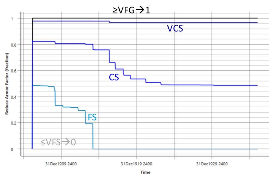
Level 6 | Level 6 includes some more detailed results and a wider suite of BSTEM results (including all of the grain-class specific results) if the model includes any BSTEM cross sections. For BSTEM variable descriptions see the Output section of the BSTEM manual and Table 41. Includes all variables from Levels 1-5. Mass (or Volume) Capacity (for every grain class) (tons/day or ft3/day) – This is the transport capacity computed by the transport function for each grain class (which is the transport HEC-RAS actually uses in its grain-class independent rout Long. Cum Mass (or Volume) Movable Limits (tons or ft3) - This is the same as the Longitudinal Cumulative Mass or Volume change in Level 1, except it excludes any bed change outside the movable bed limits. The Longitudinal Cumulative Mass (Volume) change sums the mass or volume change from the beginning of the simulation and from upstream-to-downstream, so that the downstream cross section at the last time step of the Longitudinal Cumulative Mass Curve (LCMC) is a summary of the total aggradation or degredation in that reach for the simulation. Comparing the full LCMC (or LCVC) to this one, that only reports the result in the movable bed limits, is a helpful way to differentiate between overbank and channel processes (e.g. determine what percentage of deposition is floodplain deposition or identify overbank deposition offsetting channel erosion). (Total and by grain class) Mass Subsurface (Volume): (tons or ft3) (tonnes or m3) – The sediment mass or volume (total and by grain class) in an intermediate mixing layer between the cover (which is in Level 5) and inactive layers in the Thomas and Copeland mixing methods. The Active Layer method does not have this layer. Mass Inactive (Volume): (tons or ft3) (tonnes or m3) – The sediment mass or volume (total and by grain class) in the deepest mixing layer of the control volume. The deepest mixing layer has the same name for all mixing algorithms. Hydraulic Radius – The area of the channel (the part of the cross section between the movable bed limits) divided by the wetted perimeter of the channel. Movable Elv L and Movable Elv R: (ft) (m) – These are the elevations of the movable bed limits. Tracking the MBL movement relative to the channel can be useful, but these are mainly used to track toe migration in BSTEM models. Movable Sta L and Movable Sta R: (ft) (m) – These are the stations (lateral stations of the station-elevation points) of the movable bed limits. These will remain constant unless the cross section has BSTEM parameters. Only the BSTEM algorithms move cross section station-elevation points laterally. Reduce Armor Factor (decimal between 0 and 1) – The Armor Reduction Factor determines how effective the cover layer is in the Thomas and Copeland mixing algorithms. It is the "Armoring Ratio" in Figure 217 and Figure 220. HEC-RAS multiplies the capacity deficit of each grain class by this ratio (computed from the "equivalent particle diameters" of coarser particles in the cover layer). An armor ratio of 1 is no armoring, 0 is complete armoring (for that grain class) and anything in between is partial armoring. For example, in the figure below, all the grain gravel and cobble grain classes remain unarmored throughout the simulation (RAF=1). Very Fine Sand and finer grain classes are all completely armored after the first time step (RAF=1). Three sand size classes gradually armor over time, with fine sand fully armoring (goes to zero) during the simulation and Coarse Sand eventually reducing erosion by ~50% because of armoring effects (RAF=0.5). d16 Cover/Subsurface/ Inactive Layers (mm) – The 16th percentile particles size of the specified mixing layer. Some practitioners prefer the d16 to d10 because it is two standard deviations below the mean. d84 Cover/Subsurface/ Inactive Layers (mm) The 84th percentile particles size of the specified mixing layer. Some practitioners prefer the d84 to d90 because it is two standard deviations above the mean. |

Only Customized
In general, if users Select Customized Output variables, HEC-RAS will add the selected variables to the results associated with the selected Output Level. However, this option turns off all automatic results, reporting only the results the user individually selects.