Download PDF
Download page Layer List.
Layer List
The Layers window provides a list of the layers available for display and is organized with a tree structure based on the HEC-RAS data structure and the supporting data layers needed for model evaluation – there are groups for "Features", “Geometries”, “Results”, “Map Layers”, and “Terrain”.
To interact with a layer, the layer must be Selected. The selected layer is shown in the Layers list with the Selection Color. The default selection color is magenta. In order to interact with any layer, it must be the Selected Layer.
The Selected Layer will be displayed in the Selection Color.
To change the display order of a layer, right-click on a layer and choose from the Move Layer menu item options. (Note: layers may not be moved between groups in the layer list.) Additional options available for each layer through the right click are summarized in the table below.
| Option | Description |
|---|---|
Layer Properties | Provides access to the visualization properties, feature table, and source files. Double click on the layer opens the Layer Properties. |
Open Feature Table | Provides access to the underlying feature table. |
Zoom to Layer | Zooms the Display Window to the extents of the selected layer. |
Remove Layer | Remove a layer from the Layers Window. |
Move Layer | Used to reorder the layer list and by moving the layer: To the Top, Up one Level, Down one Level, or To the Bottom of the layer list. |
Export Layer | Allows the user to export a vector data to Shapefile format for viewing in an alternative GIS. |
Open Folder in Windows Explorer | Opens Windows Explorer to location of current layer. |
Other | Other options are available specific to the layer. |
Interactive tools are available for the active layer. The layer becomes active when selected by clicking on it in the layer list. The text for the active layer will be drawn in the selection color (magenta). This active layer will be use for selecting features in the Display Window using the Select tool, animation profile information (if available), and reporting information based on the mouse position.
Layer Properties
The Layer Properties option provides access to display properties and information about the layer. Vector data and raster data both access the same properties dialog; however, the options available depend on the data type. Vector data will allow for the changing of point, line, and fill symbology. Raster data allow for the changing of the surface fill, contour, and hill shade properties. Depending on the layer type, the Layer Properties dialog will also provide access to information about the layer features and source file information. An example Layer Properties dialog is shown below.

Plot options specific to the layer shown will be will be shown in the "Additional Options" portion of the Layer Properties dialog.
Vector Data
Vector data are symbolized by points, lines, and/or fill colors which have access to their own editors. Depending on the type of layer selected, different options are available.
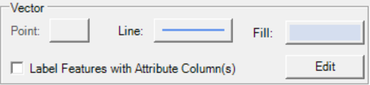
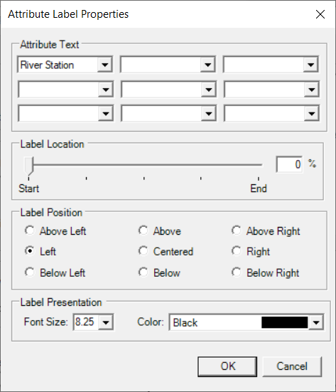
Options for vector data also allow for labeling of each feature when the "Label Features" option is checked. This will draw to the Map Window a label based on the field selected by the user. To select the labeling field and placement, click the Edit button. The Label Properties dialog, shown below, allows the user to choose the attribute, location, and presentation (font) for the label text. Fields in the attribute table are available to be selected. For lines, the Label Location defines where to place the label based on the start or end of the line.
Raster Data
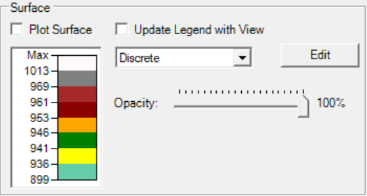
Options available for displaying surface data will be enabled for raster data. A legend for the surface fill color properties is created with corresponding layer values. The surface fill can be plotted as either a “Stretched” (interpolated) color ramp or as “Discrete” (banded) color values.
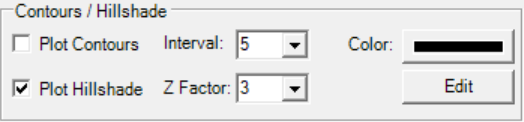
Contours and hillshade options allow for more detailed visualization of raster data. Contours are generated dynamically based on the interpolation of the raster data. Using the Hillshade option allows for shadowing of elevation data based on the angle of a light source, and can give the dataset a "3D" feel to the data. It also allows for the vertical exaggeration of the data to provide more pronounced relief.
To change the surface fill properties, select the “Edit” button. The surface fill properties dialog (shown below) allows the user to select from predefined color ramps. The predefined color ramps have a predefined range of values over which to apply colors (Depth, Velocity, Arrival Time ...). Other color ramps do not have a predefined values associated with a color (Terrain, Water Surface Elevation, …) as they are expected to be applied to layers that have a wide range of possible values. For these layers, the color ramps are applied to layer based on the minimum and maximum values in the dataset.

The colors and values in the Surface Symbol table can be changed by the user to create a new surface fill. To create a surface fill, enter the Max and Min values for the data and number of colors to interpolate over and press the Create Ramp Values button. Functionality to reverse the color ramp and to save the color ramp to the color list are available.
Features
The "Features" group contains a layer named "Profile Lines". The Profile Lines layer allows you to create lines in location you consistently are requiring results information. These lines are created and edited just as any other vector dataset. (Editing features will be discussed in detail throughout this document.) The Features group is also your RAS Mapper digital playground - you can add existing Shapefiles and create new ones to hold points, lines and polygons. New Shapefile layers can be created by right-clicking on the Features group and selecting the Create New Layer option.
Editing Tools will be discussed in detail throughout the HEC-RAS Mapper documentation, but you can start in the Geometry Data section.
Profile Lines will be discussed in the Mapping Results section.
Geometries
The “Geometries” group displays the RAS Geometry files used in the current HEC-RAS project. In addition to the normal geometry files (*.g0n), the RAS geometric data are saved to an HDF5 file format (*.g0n.hdf), processed, and displayed in RAS Mapper. For each Geometry, there will be a Layer to represent hydraulic model information. For 1D modeling there will be a layers for the River, Junctions, Flow Path Lines, Bank Lines, Cross Sections, Ineffective Flow Areas, Blocked Obstructions, Manning's n Values, and Storage Areas. For 2D modeling, there will be a 2D Flow Area layers constructed from a Perimeter polygon, Computation Points, Break Lines, and Refinement Regions. Additionally, there will be layers that are computed from the base data River Edge Lines, and the XS Interpolation Surface.
Geometry Layers creation and use will be discussed in detail in the Geometry Data section.
Results
The “Results” node displays the simulation results from each RAS Plan as saved in the RAS Plan’s output HDF5 file (*.p01.hdf). For each Plan, a copy of the geometry that was used for the simulation will be stored in the output file along with stage and flow data for each computation location. Output layers for Depth, Velocity, and Water Surface Elevation will be automatically generated within RAS Mapper for each plan.
The output layers are not stored to disk, rather they will be generated dynamically (on-the-fly) for the current map extents. Each output layer can be animated through the Animate tool. The Animate tool will work on the selected layer. To animate multiple layers, the RAS Plan must be selected. If the Plan is selected, all layers in the group (that are checked on) will be animated together. To animate all output results, select the Results group node and check on all layers to animate. Output for each Mapping Output Interval, as specified on the Unsteady Flow Plan editor, will be available for display. The current time step for the animation will be update on the display screen as well as the layer name in the Layers list. If available, the Max and Min values for the simulation will also be available for mapping. There are tools to play through the animation using the animated button. The "Tortoise" button will allow you access to another window which allows you to slow down the animation by delaying visualization of the next time-step.

Map Layers
Additional data added to the RAS Mapper (not constructed by HEC-RAS) will be added into the “Map Layers” list as background data. Data formats that are supported include Shapefile, GML, VRT, and image file formats. If the map projection has been specified and the data has a specified projection, it will be re-projected on the fly to the map projection.
Web imagery data will also be displayed under the Map Layers node. To add background imagery data, select the Project | Add Web Imagery menu item and choose from the specified list of services. The map projection for RAS Mapper must be specified when using web imagery.
Terrains
The “Terrains” node is where all Terrain layers are listed. A Terrain Layer is used by RAS Mapper for computing hydraulic properties (elevation – volume, elevation – wetted perimeter, elevation profiles, etc), inundation depths and floodplain boundaries, once it has been associated with a Geometry and Plan. Prior to using a Terrain, it must be created through the Create New Terrain Layer tool.
RAS Terrain layers will be discussed in detail in the Terrain Layer section.