Download PDF
Download page Annual Peak Record Extension - MF Eel River.
Annual Peak Record Extension - MF Eel River
The MFEelRiver_RecordExtension example demonstrates the usage of the Record Extension Analysis in order to extend a shorter annual maximum flow time series using a site with a longer period of record.
Input Data
In this example, time series representing annual maximum flow at two locations within the Eel River watershed in California are analyzed. The primary (i.e. long record) time series is from the Eel River at Scotia, CA stream gage, which has a drainage area of approximately 3113 square miles (sq mi) and a period of record from 1911 - 2021. The secondary (i.e. short record) time series is from the Middle Fork Eel River near Dos Rios, CA stream gage, which has a drainage area of approximately 745 sq mi and a period of record from 1966 - 2021. The location of these stream gages is shown in Figure 1. The time series are plotted within Figure 2 and tabulated within Table 1.
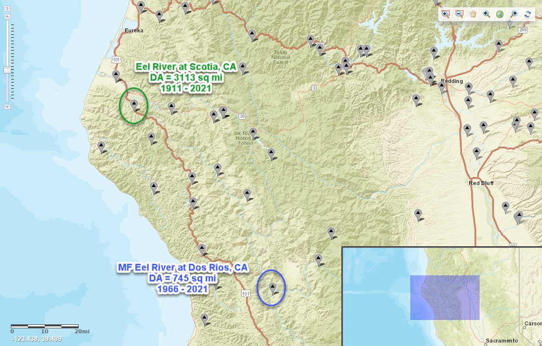
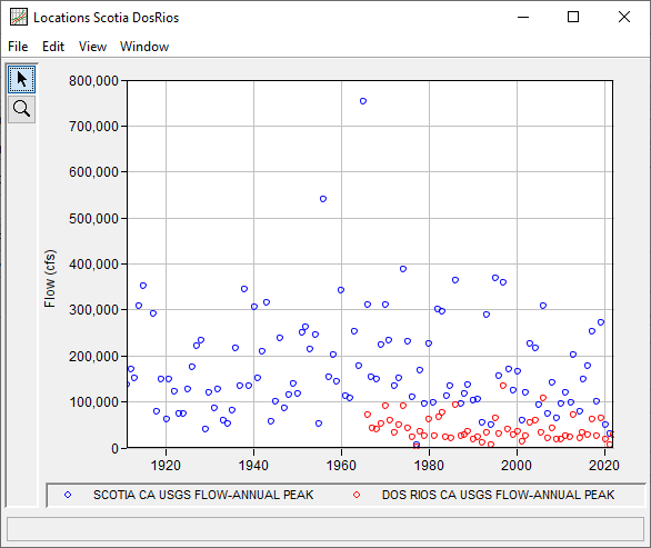
Table 1. Input Time Series for MFEelRiver_RecordExtension Example
| Date | Flow (cfs) | |
|---|---|---|
| Scotia | Dos Rios | |
| 20 Jan 1911 | 136000 | |
| 26 Jan 1912 | 170000 | |
| 18 Jan 1913 | 150000 | |
| 22 Jan 1914 | 309000 | |
| 02 Feb 1915 | 351000 | |
| 25 Feb 1917 | 292000 | |
| 07 Feb 1918 | 78600 | |
| 17 Jan 1919 | 149000 | |
| 16 Apr 1920 | 62000 | |
| 19 Nov 1920 | 148000 | |
| 19 Feb 1922 | 123000 | |
| 28 Dec 1922 | 73400 | |
| 08 Feb 1924 | 73400 | |
| 06 Feb 1925 | 127000 | |
| 04 Feb 1926 | 176000 | |
| 21 Feb 1927 | 221000 | |
| 27 Mar 1928 | 233000 | |
| 04 Feb 1929 | 41000 | |
| 15 Dec 1929 | 120000 | |
| 23 Jan 1931 | 87000 | |
| 27 Dec 1931 | 127000 | |
| 17 Mar 1933 | 58100 | |
| 29 Mar 1934 | 50900 | |
| 08 Apr 1935 | 79900 | |
| 16 Jan 1936 | 216000 | |
| 05 Feb 1937 | 134000 | |
| 11 Dec 1937 | 345000 | |
| 03 Dec 1938 | 133000 | |
| 28 Feb 1940 | 305000 | |
| 24 Dec 1940 | 150000 | |
| 06 Feb 1942 | 209000 | |
| 21 Jan 1943 | 315000 | |
| 04 Mar 1944 | 57800 | |
| 03 Feb 1945 | 99100 | |
| 27 Dec 1945 | 239000 | |
| 12 Feb 1947 | 86100 | |
| 08 Jan 1948 | 114000 | |
| 18 Mar 1949 | 140000 | |
| 18 Jan 1950 | 117000 | |
| 22 Jan 1951 | 249000 | |
| 27 Dec 1951 | 262000 | |
| 09 Jan 1953 | 215000 | |
| 17 Jan 1954 | 245000 | |
| 31 Dec 1954 | 52400 | |
| 22 Dec 1955 | 541000 | |
| 25 Feb 1957 | 153000 | |
| 25 Feb 1958 | 202000 | |
| 12 Jan 1959 | 145000 | |
| 08 Feb 1960 | 343000 | |
| 11 Feb 1961 | 113000 | |
| 14 Feb 1962 | 107000 | |
| 01 Feb 1963 | 252000 | |
| 21 Jan 1964 | 178000 | |
| 23 Dec 1964 | 752000 | |
| 04 Jan 1966 | 70200 | |
| 05 Jan 1966 | 311000 | |
| 05 Dec 1966 | 154000 | |
| 29 Jan 1967 | 42600 | |
| 14 Jan 1968 | 40000 | |
| 15 Jan 1968 | 148000 | |
| 13 Jan 1969 | 223000 | |
| 20 Jan 1969 | 52300 | |
| 23 Jan 1970 | 90500 | |
| 24 Jan 1970 | 310000 | |
| 04 Dec 1970 | 234000 | |
| 16 Jan 1971 | 59900 | |
| 23 Jan 1972 | 133000 | 33000 |
| 16 Jan 1973 | 152000 | 49200 |
| 16 Jan 1974 | 387000 | 89500 |
| 18 Mar 1975 | 231000 | |
| 25 Mar 1975 | 41700 | |
| 26 Feb 1976 | 109000 | 23700 |
| 21 Feb 1977 | 1470 | |
| 10 Mar 1977 | 5790 | |
| 09 Jan 1978 | 35800 | |
| 17 Jan 1978 | 169000 | |
| 11 Jan 1979 | 96100 | 25100 |
| 13 Jan 1980 | 61700 | |
| 14 Jan 1980 | 226000 | |
| 28 Jan 1981 | 98700 | |
| 14 Feb 1981 | 25100 | |
| 20 Dec 1981 | 300000 | |
| 16 Feb 1982 | 67000 | |
| 26 Jan 1983 | 76800 | |
| 27 Jan 1983 | 296000 | |
| 10 Nov 1983 | 23600 | |
| 09 Dec 1983 | 112000 | |
| 12 Nov 1984 | 133000 | |
| 08 Feb 1985 | 20200 | |
| 17 Feb 1986 | 364000 | 93100 |
| 12 Mar 1987 | 25000 | |
| 13 Mar 1987 | 94500 | |
| 10 Dec 1987 | 118000 | 27000 |
| 23 Nov 1988 | 137000 | 33900 |
| 08 Jan 1990 | 102000 | 18800 |
| 04 Mar 1991 | 22700 | |
| 05 Mar 1991 | 105000 | |
| 20 Feb 1992 | 54200 | 10800 |
| 20 Jan 1993 | 33700 | |
| 21 Jan 1993 | 290000 | |
| 23 Jan 1994 | 7220 | |
| 24 Jan 1994 | 48500 | |
| 09 Jan 1995 | 368000 | 65000 |
| 12 Dec 1995 | 155000 | 30000 |
| 01 Jan 1997 | 360000 | 135000 |
| 12 Jan 1998 | 40300 | |
| 17 Jan 1998 | 170000 | |
| 08 Feb 1999 | 125000 | |
| 09 Feb 1999 | 27500 | |
| 14 Feb 2000 | 166000 | 34600 |
| 05 Mar 2001 | 59000 | 13000 |
| 02 Jan 2002 | 119000 | 24800 |
| 16 Dec 2002 | 226000 | 53700 |
| 17 Feb 2004 | 59700 | |
| 18 Feb 2004 | 217000 | |
| 08 Dec 2004 | 93800 | |
| 18 May 2005 | 32600 | |
| 30 Dec 2005 | 107000 | |
| 31 Dec 2005 | 307000 | |
| 26 Dec 2006 | 20600 | |
| 27 Dec 2006 | 74900 | |
| 04 Jan 2008 | 42500 | |
| 05 Jan 2008 | 142000 | |
| 24 Feb 2009 | 64300 | |
| 02 Mar 2009 | 18300 | |
| 25 Jan 2010 | 17700 | |
| 26 Jan 2010 | 94400 | |
| 29 Dec 2010 | 119000 | 24700 |
| 21 Jan 2012 | 21800 | |
| 28 Mar 2012 | 98000 | |
| 02 Dec 2012 | 202000 | 70300 |
| 29 Mar 2014 | 79500 | 19400 |
| 11 Dec 2014 | 33000 | |
| 07 Feb 2015 | 148000 | |
| 18 Jan 2016 | 177000 | 27000 |
| 08 Jan 2017 | 61600 | |
| 11 Jan 2017 | 252000 | |
| 07 Apr 2018 | 101000 | 26000 |
| 27 Feb 2019 | 272000 | 62900 |
| 26 Jan 2020 | 50200 | 17500 |
| 02 Feb 2021 | 30100 | 5560 |
| 24 Oct 2021 | 28400 | |
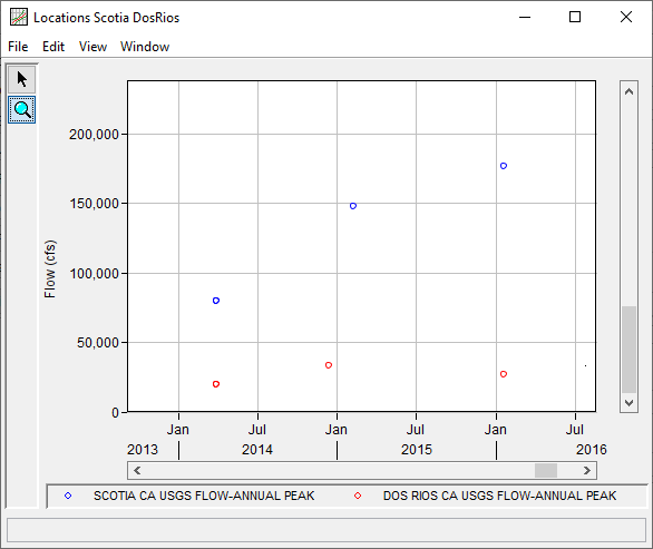
Inspecting the 56 years of overlapping data, it is evident that some of the annual peaks are not "truly" concurrent (i.e. the annual peak for a given water year at the long term site occurred during a different runoff event when compared to the short term site), as shown in Figure 4. Per Bulletin 17C: "For the purposes of record extension, concurrent flood peaks are those that occurred in the same water year, not on the same flood event." As such, the entire overlapping record was considered concurrent within this example.
The Correlation Analysis within HEC-SSP can be used to identify any peak flow data points that are many days apart. For an example of how to create a Correlation Analysis for this purpose, see Using a Correlation Analysis to Select a Suitable Nearby Gage for Record Extension.
General Tab
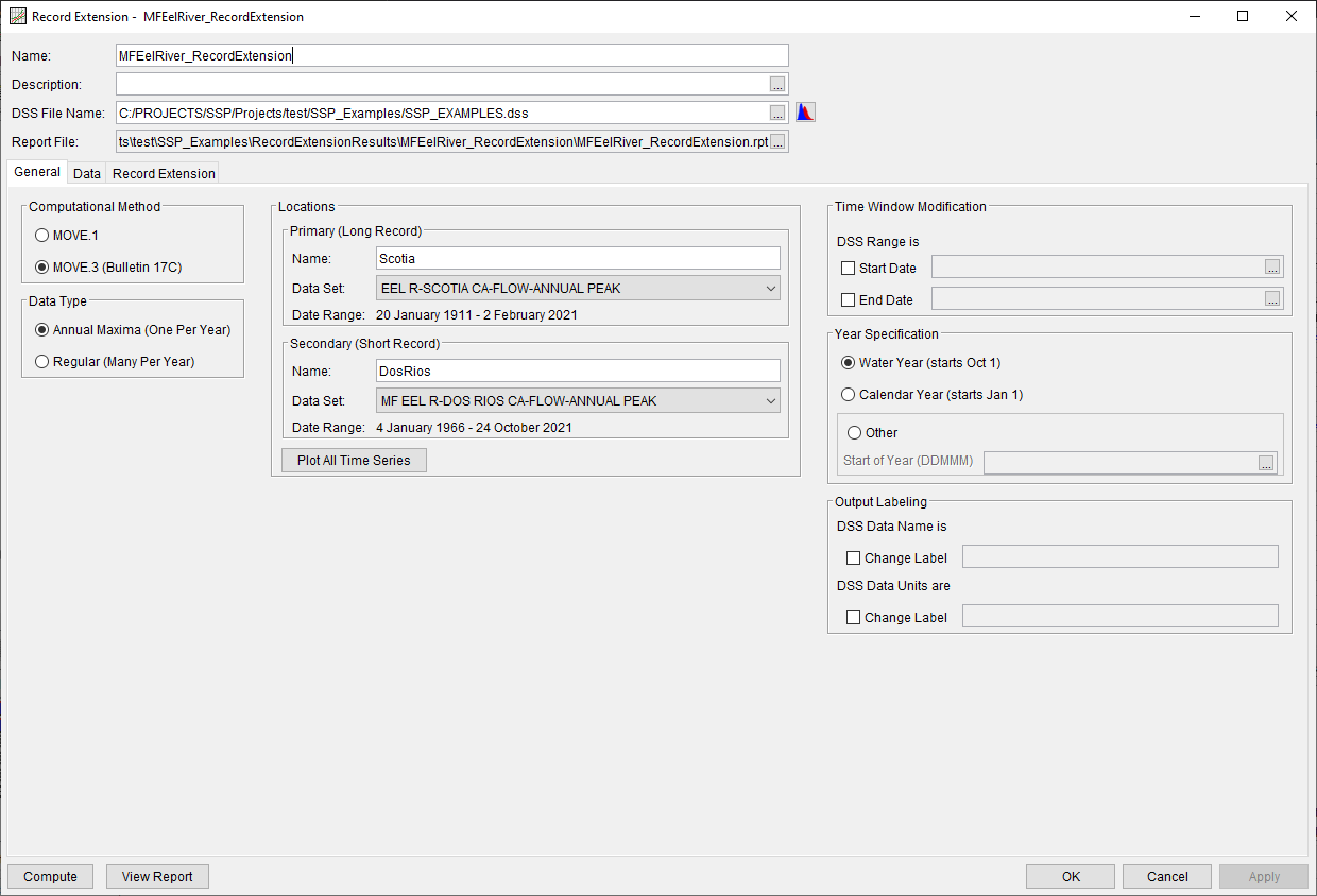
A Record Extension Analysis has been developed for this example. To open the analysis, either double-click on the analysis labeled MFEelRiver_RecordExtension from the study explorer or from the Analysis menu select open, then select MFEelRiver_RecordExtension from the list of available analyses. When MFEelRiver_RecordExtension is opened, the General tab within the Record Extension Analysis editor will appear as shown in Figure 4. For this analysis, the MOVE.3 (Bulletin 17C) computational method and the Annual Maximum (One Per Year) data type was selected. The Scotia time series was selected as the Primary (Long Record) while the Dos Rios time series was selected as the Secondary (Short Record). The default Year Specification (Water Year) was left unchanged. No modifications were made to the time window or the output labeling.
Data Tab
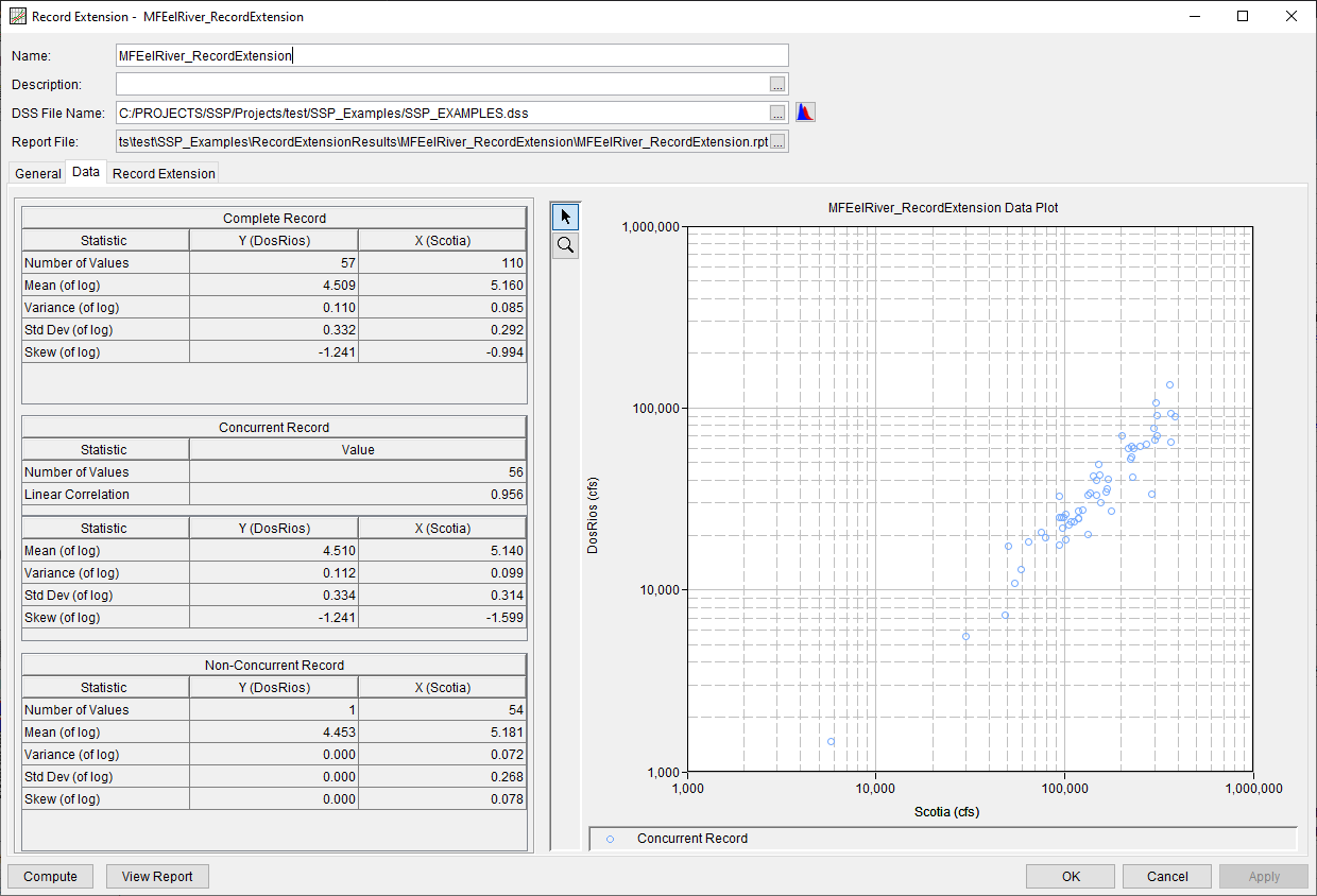
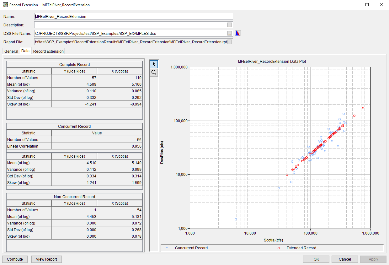
The Data tab contains several tables detailing the complete, concurrent (i.e. overlapping), and non-concurrent (i.e. non-overlapping) records. Additionally, a plot showing the concurrent record is included. The primary record (Scotia) is shown on the x-axis while the secondary record (Dos Rios) is shown on the y-axis. Prior to a successful compute, the plot will only contain the concurrent record (blue circles), as shown in Figure 5. Following a successful compute, the extended record (red circles) will be added to the plot, as shown in Figure 6.
Computing the Analysis
Once all of the General information has been selected and the data reviewed on the Data tab, the user can press the Compute button to perform the analysis. Once the computations have been completed, a message window will open stating Compute Complete.
The Record Extension Analysis will use all values within the concurrent time period when computing correlation coefficients, estimators for augmentation, and the extended record. No values will be removed from consideration even though they may not have resulted from the same runoff event, as was mentioned above.
Record Extension Tab
The Record Extension tab contains several tables detailing the Matalas-Jacobs Estimators (MJ-Mean and MJ-Variance), the Estimators for Augmentation, and statistics of the extended record. Additionally, a plot showing the input time series is included. Prior to a successful compute, the plot will only contain the primary record (Scotia; green circles) and the secondary record (Dos Rios; blue circles), as shown in Figure 7. Following a successful compute, the extended record (red circles) will be added to the plot, as shown in Figure 8.
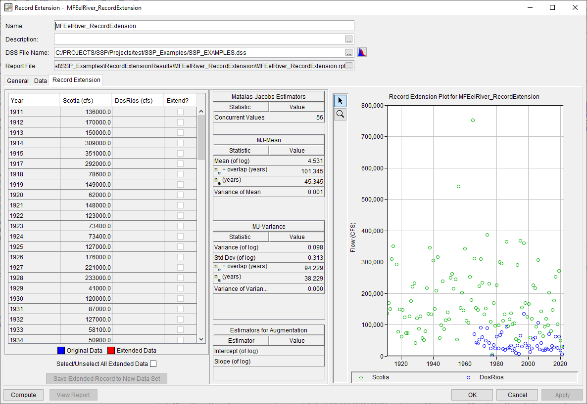
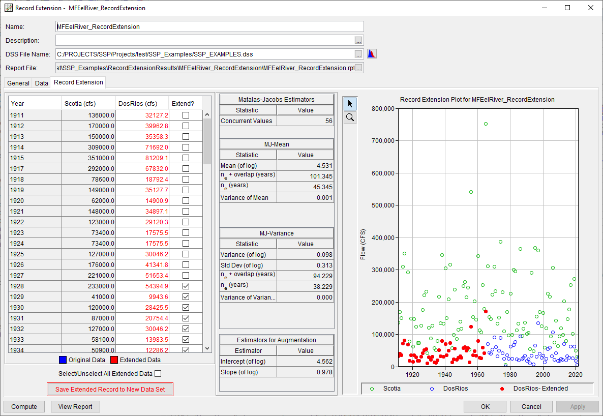
Since this example made use of the MOVE.3 (Bulletin 17C) computational method and the Annual Maximum (One Per Year) data type, following a successful compute, the effective record length (ne) of the variance will be used to select data for extension. Specifically, the most recent ne years will be selected and the Save Extended Record to New Data Set button will become enabled.
The user may select a different portion of the extended record to save to a new data set. However, the Estimators for Augmentation were computed using the most recent ne years. As such, choosing a different portion of the extended record will not result in the Matalas-Jacobs estimators being reproduced within the extended record. It is recommended that the user selects the default extended record when saving to a new data set.
The Save Extended Record to New Data Set button will only be active following a successful compute.
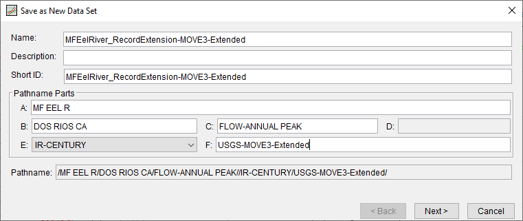
When the Save Extended Record to New Data Set is clicked, a dialog will be presented allowing for the definition of a Name, Description, Short ID, and DSS Pathname Parts for the new data set, as shown within Figure 9.
Upon clicking the Next button, a Save As New Data Set Summary dialog will be shown allowing the user to review the metadata of the new data set as well as a tabulation and plot of the data that is about to be imported, as shown in Figure 10.
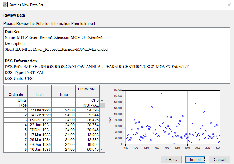
Once the extended record is saved to a new data set, it can be used to compute updated flow-frequency information. An example of this type of application is shown here.
Report File
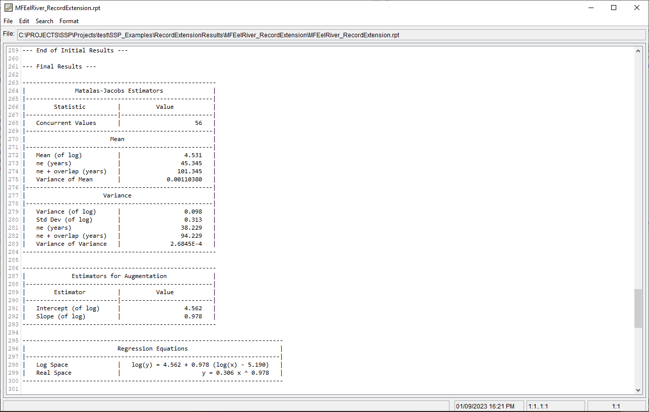
In addition to the tabular and graphical results, there is a report file that echoes the input data, selected computational options, and results. To review the report file, press the View Report button at the bottom of the analysis window. When this button is selected a text viewer will open the report file and display it on the screen, as shown in Figure 11.
Different types and amounts of information will show up in the report file depending on the data and the options that have been selected for the analysis.
