Download PDF
Download page R/RStudio Crash Course Workshop.
R/RStudio Crash Course Workshop

Software
CRAN R version 4.4.3 or newer
RStudio version 2024.12.1 or newer
This workshop assumes you have no prior experience in using either the R programming language, or the RStudio integrated development environment. The instructions will help you get R and RStudio installed and configured, and then begin to learn the foundations of working with R. Both R and RStudio are CIO/G-6 approved software for use on USACE hardware, and they are freeware, meaning they do not require any purchasing or licensing to work.
The following major tasks will serve as an outline for the workshop:
- Installing and Configuring R and RStudio
- Getting Started in RStudio
- Introduction to R Fundamentals
- Running Your First R Script
Read through the documentation linked in Tasks 1-3.
In Task 4, you will run the provided script.
Task 1. Installing and Configuring R and RStudio
First, follow these instructions: Installing and Configuring R and RStudio
Task 2. Getting Started in RStudio
R is a programming language geared towards statistical analysis. It simplifies a lot of common statistical tasks and makes it easier to generate statistical graphics. Its capabilities are expanded by open source libraries called packages. RStudio is an IDE, which is a tool used to facilitate development of code in a programming language.
First, start up RStudio and then take a quick tour of its user interface with this guide: Introduction to RStudio.
Task 3. Introduction to R Fundamentals
There are several features fundamental to working with R that might make it different than other programming languages. Read the following page to become familiar with some of these fundamentals before beginning the workshop: Introduction to R.
Task 4. Running Your First R Script
Set Working Directory
First, set your working directory. In the lower right window, select the Files tab. Select the file brower (...) and navigate to the folder containing the starting data for this workshop. You must select a folder for the working directory.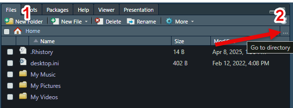
On the Files tab, select the More menu to open a drop-down menu. Select Set As Working Directory. 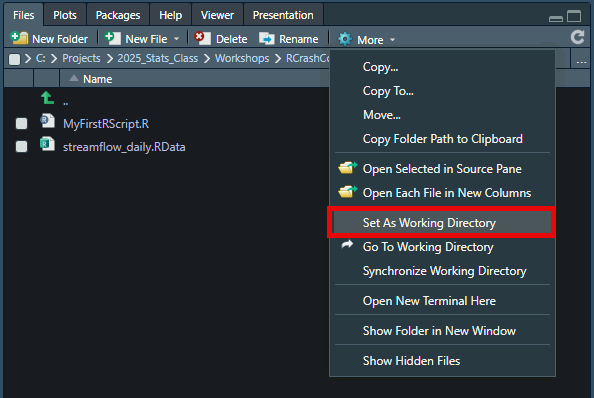
Save both files linked above (MyFirstRScript.R and streamflow_daily.RData) to your working directory. Select File | Open File... and open the MyFirstRScript.R script.
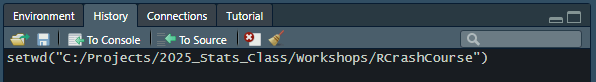
In the upper right window, select the History tab. You should see a command ("setwd") in the terminal. This sets the working directory to the directory noted inside the function.
On the History tab, select that last command (setwd). The row containing the command should change colors when it is selected. Press the To Source button to add it to your script on line 2.
A working directory allows you to set the root directory for relative paths, and lets you access files by name in the working directory without needing to specify a full file path.
Set Working Directory
# Set working directory
setwd("<Your file directory here>")To specify a directory path in R, you have two options:
- Use two backslashes:
setwd("C:\\Projects\\ILoveR") - Use a forward slash:
setwd("C:/Projects/ILoveR")
Using a single backslash will result in an error since a single backslash is used to denote an escape character (e.g. \n is the escape character for a new line).
Install Packages
Packages can be installed using the package installation tool as described in Installing and Configuring R and RStudio. There are three libraries attached to the script: tidyverse, dataRetrieval, and moments. As a result, you will be prompted to install the packages at the top of the script. Click Install (shown below in the red box) to install the packages.

In the bottom pane, click on the Background Jobs tab. You will see text appearing as the packages are installed. Wait until package installation is complete and you see the following text:
✔ Packages successfully installed.
Attach Packages
Libraries should be attached at the top of the script using the library function.
The dataRetrieval package is used to download U.S. Geological Survey hydrologic data.
The tidyverse package is a set of packages that are among the most commonly used R packages. The ggplot2 package is contained within the tidyverse package. We will use ggplot2 for data visualization later in this tutorial.
The moments package is used to compute mathematical moments.
Run lines 5-7 to attach packages.
Attach Packages
# Attach packages
library(tidyverse)
library(dataRetrieval)
library(moments)
Define Custom Functions
Review the Functions section of the Introduction to R page for additional information. An R function is created using the keyword function. A function in R has the following general syntax:
Function Syntax
function_name <- function(<arg1>, <arg2>, ...) {
 # Function body
}A function is comprised of the following components:
- Function name: The name of the function. The function is stored in R environment as an object with this name.
- Arguments: Arguments are optional placeholders. When a function is called, you pass a value to the argument.
- Function body: The function body contains statements used to perform a specific task.
- Return value: The return value of a function is the last expression in the function body.
Variables defined within the function body are local variables. These variables exist only within the function. A function can invoke another function.
In this code block, we will define 2 custom functions: weibull_pp and wy.
The weibull_pp function computes the Weibull plotting position using the formula P = \frac {i}{n + 1} where i is the rank of the data and n is the number of data values. In R, the rank function assigns a rank of 1 to the smallest value. Therefore, this version of the Weibull plotting position describes empirical non-exceedance probability.
The wy function computes the water year (WY) based on a date. In the United States, a WY spans October 1 through September 30 of the following year and is named by the year in which the measurements end (e.g., WY 2022 spans October 1, 2021 through September 30, 2022). The functions month and year come from the lubridate package, which is one of several libraries under the tidyverse umbrella.
Run lines 9-25.
Define Custom Functions
# Custom functions

# Computes the Weibull plotting position (empirical non-exceedance probability)
weibull_pp <- function(x) {
  n <- length(x)
  i <- rank(x) # In R, rank = 1 corresponds to the smallest value
  return(i / (n+1))
}

# Computes water year
wy <- function(date) {
  ifelse(month(date) > 9, year(date)+1, year(date))
}Get Gage Site Info Using the dataRetrieval Package
The dataRetrival package readNWISsite function imports site information from USGS based on a site number. Run lines 26-30.
Get Gage Site Info Using the dataRetrieval Package
# Get gage site info
siteNo <- "11266500" # Merced River at Pohono Bridge near Yosemite, CA
siteInfo <- readNWISsite(siteNo)
siteInfoQUESTION 1. What information is provided by the readNWISsite function?
The function returns the following information:
| Name | Type | Description |
| agency_cd | character | The NWIS code for the agency reporting the data |
| site_no | character | The USGS site number |
| station_nm | character | Site name |
| site_tp_cd | character | Site type |
| lat_va | numeric | DMS latitude |
| long_va | numeric | DMS longitude |
| dec_lat_va | numeric | Decimal latitude |
| dec_long_va | numeric | Decimal longitude |
| coord_meth_cd | character | Latitude-longitude method |
| coord_acy_cd | character | Latitude-longitude accuracy |
| coord_datum_cd | character | Latitude-longitude datum |
| dec_coord_datum_cd | character | Decimal Latitude-longitude datum |
| district_cd | character | District code |
| state_cd | character | State code |
| county_cd | character | County code |
| country_cd | character | Country code |
| land_net_ds | character | Land net location description |
| map_nm | character | Name of location map |
| map_scale_fc | character | Scale of location map |
| alt_va | numeric | Altitude of Gage/land surface |
| alt_meth_cd | character | Method altitude determined |
| alt_acy_va | numeric | Altitude accuracy |
| alt_datum_cd | character | Altitude datum |
| huc_cd | character | Hydrologic unit code |
| basin_cd | character | Drainage basin code |
| topo_cd | character | Topographic setting code |
| instruments_cd | character | Flags for instruments at site |
| construction_dt | character | Date of first construction |
| inventory_dt | character | Date site established or inventoried |
| drain_area_va | numeric | Drainage area |
| contrib_drain_area_va | numeric | Contributing drainage area |
| tz_cd | character | Time Zone abbreviation |
| local_time_fg | character | Site honors Daylight Savings Time |
| reliability_cd | character | Data reliability code |
| gw_file_cd | character | Data-other GW files |
| nat_aqfr_cd | character | National aquifer code |
| aqfr_cd | character | Local aquifer code |
| aqfr_type_cd | character | Local aquifer type code |
| well_depth_va | numeric | Well depth |
| hole_depth_va | numeric | Hole depth |
| depth_src_cd | character | Source of depth data |
| project_no | character | Project number |
However, not every field will return a value for every gage.
Load an *.RData File of Mean Daily Flow
The load function is used to load R objects. The head function is used to display the first n rows of the provided data frame. By default, n = 6.
Run lines 31-34.
Load an *.RData File of Mean Daily Flow
# Load the *.RData file containing mean daily streamflow for WY 1917-2022
load("streamflow_daily.RData")
head(streamflow_daily)You should see the following output in the Console:
  agency_cd  site_no       Date Flow Flow_cd
1      USGS 11266500 1916-10-01  285       A
2      USGS 11266500 1916-10-02  285       A
3      USGS 11266500 1916-10-03  285       A
4      USGS 11266500 1916-10-04  285       A
5      USGS 11266500 1916-10-05  285       A
6 USGS 11266500 1916-10-06 285 AUse the dataRetrieval Package to Download Annual Peak Flows
The dataRetrieval package readNWISpeak function is used to download the annual peak flows at USGS 11266500 Merced River at Pohono Bridge near Yosemite, CA.
Run lines 35-38.
Use the dataRetrieval Package to Download Annual Peak Flows
# Read peak flows
peak_flow_table <- readNWISpeak(siteNumbers = siteNo)
head(peak_flow_table)You should see the following output in the Console:
  agency_cd  site_no    peak_dt peak_tm peak_va peak_cd gage_ht gage_ht_cd year_last_pk ag_dt ag_tm ag_gage_ht ag_gage_ht_cd peak_dateTime
1      USGS 11266500 1917-06-10    <NA>    5880    <NA>    8.75       <NA>           NA  <NA>  <NA>         NA          <NA>          <NA>
2      USGS 11266500 1918-06-12    <NA>    4000    <NA>    7.05       <NA>           NA  <NA>  <NA>         NA          <NA>          <NA>
3      USGS 11266500 1919-05-29    <NA>    6150    <NA>    9.80       <NA>           NA  <NA>  <NA>         NA          <NA>          <NA>
4      USGS 11266500 1920-05-20    <NA>    5050    <NA>    8.80       <NA>           NA  <NA>  <NA>         NA          <NA>          <NA>
5      USGS 11266500 1921-06-11    <NA>    4610    <NA>    8.40       <NA>           NA  <NA>  <NA>         NA          <NA>          <NA>
6 USGS 11266500 1922-06-05 <NA> 6370 <NA> 10.00 <NA> NA <NA> <NA> NA <NA> <NA>Apply Custom Functions and tidyverse Functions to the Annual Peak Flows
We will assign the peak_flow_table dataframe to a new variable named ams. We will add two columns, named wy and weibull_pp, using the dplyr package mutate function. The values of these columns are computed by calling the custom functions wy and weibull_pp. Finally, we select the peak_dt, peak_va, wy, and weibull_pp columns using the dplyr package select function and assign those to the ams variable.
Run lines 39-49.
Operators
The %>% is the pipe operator. The pipe operator is a mechanism for chaining commands together. The operator will forward a value, or the result of an expression, into the next function call/expression.
The double colon operator, ::, is used to access a specific function from a package (package::function). The code dplyr::select accesses the select function from the dplyr package.
The double colon operator is needed because different packages have functions with the same name but different functionality. The double colon operator allows us to specify a particular function that we want to use. Without a specific call, the function from the most recently loaded package masks the other functions of the same name from different packages.
Apply Custom and tidyverse Functions to Annual Peak Flows
# Create new dataframe named ams from the existing peak_flow_table dataframe
# Add columns for WY and Weibull plotting position
# Select the peak flow, WY, and Weibull PP columns
ams <- peak_flow_table %>%
  mutate(wy = wy(peak_dt),
         weibull_pp = weibull_pp(peak_va)) %>% # Add columns for WY and Weibull PP; call user-defined functions wy and weibull_pp
  dplyr::select(peak_dt, peak_va, wy, weibull_pp)

# Notice that the ams dataframe contains only peak_dt, peak_va, wy, and weibull_pp columns
head(ams)You should see the following output in the Console:
     peak_dt peak_va   wy weibull_pp
1 1917-06-10    5880 1917  0.6635514
2 1918-06-12    4000 1918  0.3738318
3 1919-05-29    6150 1919  0.6915888
4 1920-05-20    5050 1920  0.5887850
5 1921-06-11    4610 1921  0.4859813
6 1922-06-05 6370 1922 0.7149533Compute Summary Statistics for All Season, January, and May Mean Daily Flows
We will compute a handful of summary statistics on the mean daily streamflow. We will compute the following summary statistics for the all season, January, and May streamflows: mean, maximum, minimum, range, interquartile range, coefficient of variation, and skewness.
Run lines 50-89.
Compute Summary Statistics for All Season, January, and May Mean Daily Flows
# Compute summary statistics for all seasons
summary_stats_all_season <- streamflow_daily %>%
  summarise(mean = mean(Flow), # Compute mean of daily average flows
            max = max(Flow), # Compute maximum of daily average flows
            min = min(Flow), # Compute minimum of daily average flows
            range = max - min, # Compute range of daily average flows
            iqr = IQR(Flow), # Compute interquartile range: IQR = Q3 - Q1 (3rd quartile - 1st quartile)
            cv = sd(Flow)/mean, # Compute coefficient of variation: cov = standard deviation/mean
            skewness = moments::skewness(Flow))

# Subset daily streamflow to January and May flows
jan_flows <- subset(streamflow_daily, month(Date) == 1) # Keep all flows that occurred during January (month = 1)
may_flows <- subset(streamflow_daily, month(Date) == 5) # Keep all flows that occurred during May (month = 5)

# Compute summary statistics for all January flows in the period of record
summary_stats_jan <- jan_flows %>%
  summarise(mean = mean(Flow),
            max = max(Flow),
            min = min(Flow),
            range = max - min,
            iqr = IQR(Flow),
            cv = sd(Flow)/mean,
            skewness = moments::skewness(Flow))

# Compute summary statistics for all May flows in the period of record
summary_stats_may <- may_flows %>%
  summarise(mean = mean(Flow),
            max = max(Flow),
            min = min(Flow),
            range = max - min,
            iqr = IQR(Flow),
            cv = sd(Flow)/mean,
            skewness = moments::skewness(Flow))

# Bind rows into a single summary statistics table
summary_stats <- rbind(all = summary_stats_all_season,
                       jan = summary_stats_jan,
                       may = summary_stats_may)
summary_statsYou should see the following output in the Console:
         mean   max   min   range    iqr       cv  skewness
all  623.9755 21000   5.4 20994.6  642.0 1.6520261  3.149698
jan  210.2115 21000  14.0 20986.0  167.0 2.4991858 23.595191
may 2321.3287 9760 198.0 9562.0 1797.5 0.5774552 1.030760QUESTION 2. Comment on the differences in flow magnitudes and summary statistics between the all season, January, and May datasets.
The maximum mean daily flow for the all season and January time frames are the same (21,000 cfs) indicating that the maximum flow during the period of record occurred in January.
The minimum flow in January is substantially lower than the minimum flow in May but the maximum flow in January is substantially higher than the maximum flow in May.
The range, interquartile range, and coefficient of variation are all measures of spread, or dispersion. The range of flows during January (20,986 cfs) is nearly the same as the all season range (20,995 cfs). Both these ranges are much larger than the May flow range (9,562 cfs).
The interquartile range is the difference between the third quartile (the 75th percentile) and first quartile (25th percentile). The range of January flows is really large but the interquartile range is much smaller than that of the May flows. This indicates that the middle 50% of January flows doesn't exhibit as much spread as the middle 50% of May flows but the highest and lowest flow values exhibit a much wider spread than the maximum and minimum May flows.
The coefficient of variation is the ratio of the standard deviation to the mean and is a standardized measure of dispersion. The January flows have the highest coefficient of dispersion (2.50), followed by the all season flows (1.65) and the May flows (0.58).
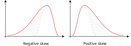
Skewness is a measure of distribution asymmetry. For example, the skewness of a normal distribution is zero. Streamflow is typically characterized by a positive skewness value, indicating a long right tail. All three skewness values are positive. The January flow skewness value is extremely positive (23.6), indicating a very heavy right-tailed distribution.
Plot the Mean Daily Hydrograph and Annual Peak Flows
This code block uses the ggplot2 package (one of the tidyverse packages) for data visualization. We can add additional commands to ggplot objects using the + operator. Think of ggplot objects as buildable.
Run lines 90-100.
Plot the Mean Daily Hydrograph and Annual Peak Flows
# Plot mean daily hydrograph
ts_plot <-
ggplot(streamflow_daily, aes(x = Date, y = Flow)) +
geom_line() + # Plot hydrograph as a line
xlab("Date") + # Add x-axis label
ylab("Mean Daily Flow (cfs)") # Add y-axis label
# Add annual peak flow values to hydrograph plot
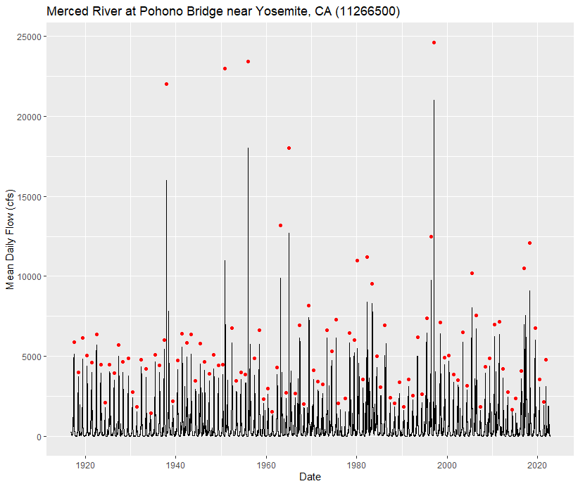
ts_plot + geom_point(data = ams, aes(x = peak_dt, y = peak_va), colour = "red") + # Plot AMS as points
labs(title = "Merced River at Pohono Bridge near Yosemite, CA (11266500)") # Add plot titleYou should see the following plot in the lower right panel under the Plots tab:
Plot the All Season Flow Duration Curve
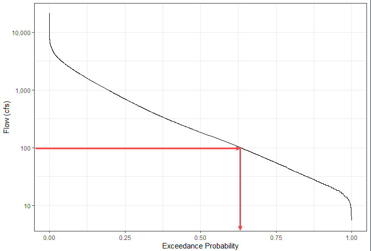
A flow duration curve shows the percentage of time that a specific discharge value is equaled or exceeded. Flow duration curves are typically computed using mean daily data. The exceedance probability is computed as P = \frac {i}{n + 1} where i is the rank of the data (i = 1 is the largest value) and n is the number of data values. This equation should look familiar (Weibull plotting position) but now i = 1 corresponds to the largest value instead of the smallest value. Instead of using the custom function weibull_pp, use the following code to add a column to the streamflow_daily data frame. Notice that we could have computed the Weibull plotting position this way instead of defining a custom function. We apply a negative sign in front of the flow values so that i = 1 corresponds to the largest flow value.
Run lines 101-112.
Plot the All Season Flow Duration Curve
# Compute exceedance probability for flow duration curve
streamflow_daily <- streamflow_daily %>%
  mutate(exPr = rank(-Flow)/(nrow(streamflow_daily) + 1))

# Plot flow duration curve
ggplot(streamflow_daily, aes(x = exPr, y = Flow)) +
  geom_line() +
  scale_y_log10(labels = scales::comma) +
  xlab("Exceedance Probability") +
  ylab("Flow (cfs)") +
theme_bw() # Change theme to black and whiteQUESTION 3. What percentage of the time is a discharge of 100 cfs equaled or exceeded at this site?
A discharge of 100 cfs is equaled or exceeded approximately 63% of the time (based on the period analyzed).
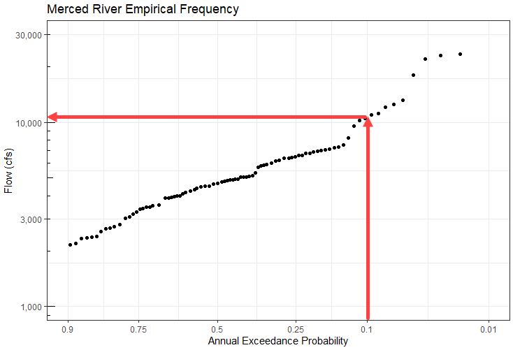
Plot Empirical Frequency of the Annual Peak Flows
The following code plots annual peak flows against annual exceedance probability (computed from the Weibull plotting position formula).
Run lines 113-128.
Plot Empirical Frequency of the Annual Peak Flows
# Define non-exceedance probability breaks for plot
pbreaks <- c(0.001, 0.01, 0.10, 0.25, 0.50, 0.75, 0.90, 0.99, 0.99)

ggplot(ams, aes(x = weibull_pp, y = peak_va)) +
  geom_point() +
  scale_x_continuous("Annual Exceedance Probability",
                     trans = scales::probability_trans("norm"), # Applies normal transformation to x-axis
                     breaks = 1-pbreaks, # Defines x-axis breaks based on specific exceedance probabilities (1 - non-exceedance probabilities)
                     labels = prettyNum(pbreaks), # Changes formatting of x-axis labels
                     limits = c(0.1, 0.99)) + # Set x-axis limits
  scale_y_log10(labels = scales::comma,
                limits = c(1000, 30000)) + # Add comma to labels on y-axis, set y-axis limits
  ylab("Flow (cfs)") +
  theme_bw() +
  annotation_logticks(sides = "l") + # Add log tick marks for readability
labs(title = "Merced River Empirical Frequency")QUESTION 4. What discharge corresponds to an annual exceedance probability (AEP) of 10%?
A discharge of 11,000 cfs has an AEP of approximately 10%, or a 1/10 chance of occurring in any given year.